Step function (original) (raw)

From Wikipedia, the free encyclopedia

Linear combination of indicator functions of real intervals

This article is about a piecewise constant function. For the unit step function, see Heaviside step function.

In mathematics, a function on the real numbers is called a step function if it can be written as a finite linear combination of indicator functions of intervals. Informally speaking, a step function is a piecewise constant function having only finitely many pieces.

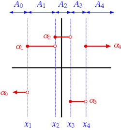
An example of step functions (the red graph). In this function, each constant subfunction with a function value αi (i = 0, 1, 2, ...) is defined by an interval Ai and intervals are distinguished by points xj (j = 1, 2, ...). This particular step function is right-continuous.

Definition and first consequences

[edit]

A function f : R → R {\displaystyle f\colon \mathbb {R} \rightarrow \mathbb {R} } $f\colon \mathbb {R} \rightarrow \mathbb {R}$ is called a step function if it can be written as [_citation needed_]

f ( x ) = ∑ i = 0 n α i χ A i ( x ) {\displaystyle f(x)=\sum \limits _{i=0}^{n}\alpha _{i}\chi _{A_{i}}(x)} $f(x)=\sum \limits _{i=0}^{n}\alpha _{i}\chi _{A_{i}}(x)$ , for all real numbers x {\displaystyle x} $x$

where n ≥ 0 {\displaystyle n\geq 0} $n\geq 0$ , α i {\displaystyle \alpha _{i}} $\alpha _{i}$ are real numbers, A i {\displaystyle A_{i}} $A_{i}$ are intervals, and χ A {\displaystyle \chi _{A}} $\chi _{A}$ is the indicator function of A {\displaystyle A} $A$ :

χ A ( x ) = { 1 if x ∈ A 0 if x ∉ A {\displaystyle \chi _{A}(x)={\begin{cases}1&{\text{if }}x\in A\\0&{\text{if }}x\notin A\\\end{cases}}} $\chi _{A}(x)={\begin{cases}1&{\text{if }}x\in A\\0&{\text{if }}x\notin A\\\end{cases}}$

In this definition, the intervals A i {\displaystyle A_{i}} $A_{i}$ can be assumed to have the following two properties:

The intervals are pairwise disjoint: A i ∩ A j = ∅ {\displaystyle A_{i}\cap A_{j}=\emptyset } $A_{i}\cap A_{j}=\emptyset$ for i ≠ j {\displaystyle i\neq j} $i\neq j$
The union of the intervals is the entire real line: ⋃ i = 0 n A i = R . {\displaystyle \bigcup _{i=0}^{n}A_{i}=\mathbb {R} .} $\bigcup _{i=0}^{n}A_{i}=\mathbb {R} .$

Indeed, if that is not the case to start with, a different set of intervals can be picked for which these assumptions hold. For example, the step function

f = 4 χ [ − 5 , 1 ) + 3 χ ( 0 , 6 ) {\displaystyle f=4\chi _{[-5,1)}+3\chi _{(0,6)}} ![{\displaystyle f=4\chi _{-5,1)}+3\chi _{(0,6)}}

can be written as

f = 0 χ ( − ∞ , − 5 ) + 4 χ [ − 5 , 0 ] + 7 χ ( 0 , 1 ) + 3 χ [ 1 , 6 ) + 0 χ [ 6 , ∞ ) . {\displaystyle f=0\chi _{(-\infty ,-5)}+4\chi _{[-5,0]}+7\chi _{(0,1)}+3\chi _{[1,6)}+0\chi _{[6,\infty )}.} ![{\displaystyle f=0\chi _{(-\infty ,-5)}+4\chi _{[-5,0]}+7\chi _{(0,1)}+3\chi _{[1,6)}+0\chi _{6,\infty )}.}

Variations in the definition

[edit]

Sometimes, the intervals are required to be right-open[1] or allowed to be singleton.[2] The condition that the collection of intervals must be finite is often dropped, especially in school mathematics,[3][4][5] though it must still be locally finite, resulting in the definition of piecewise constant functions.

The Heaviside step function is an often-used step function.

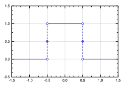
The rectangular function, the next simplest step function.

The rectangular function, the normalized boxcar function, is used to model a unit pulse.
The integer part function is not a step function according to the definition of this article, since it has an infinite number of intervals. However, some authors[6] also define step functions with an infinite number of intervals.[6]
The sum and product of two step functions is again a step function. The product of a step function with a number is also a step function. As such, the step functions form an algebra over the real numbers.
A step function takes only a finite number of values. If the intervals A i , {\displaystyle A_{i},} $A_{i},$ for i = 0 , 1 , … , n {\displaystyle i=0,1,\dots ,n} $i=0,1,\dots ,n$ in the above definition of the step function are disjoint and their union is the real line, then f ( x ) = α i {\displaystyle f(x)=\alpha _{i}} $f(x)=\alpha _{i}$ for all x ∈ A i . {\displaystyle x\in A_{i}.} $x\in A_{i}.$
The definite integral of a step function is a piecewise linear function.
The Lebesgue integral of a step function f = ∑ i = 0 n α i χ A i {\displaystyle \textstyle f=\sum _{i=0}^{n}\alpha _{i}\chi _{A_{i}}} $\textstyle f=\sum _{i=0}^{n}\alpha _{i}\chi _{A_{i}}$ is ∫ f d x = ∑ i = 0 n α i ℓ ( A i ) , {\displaystyle \textstyle \int f\,dx=\sum _{i=0}^{n}\alpha _{i}\ell (A_{i}),} $\textstyle \int f\,dx=\sum _{i=0}^{n}\alpha _{i}\ell (A_{i}),$ where ℓ ( A ) {\displaystyle \ell (A)} $\ell (A)$ is the length of the interval A {\displaystyle A} $A$ , and it is assumed here that all intervals A i {\displaystyle A_{i}} $A_{i}$ have finite length. In fact, this equality (viewed as a definition) can be the first step in constructing the Lebesgue integral.[7]
A discrete random variable is sometimes defined as a random variable whose cumulative distribution function is piecewise constant.[8] In this case, it is locally a step function (globally, it may have an infinite number of steps). Usually however, any random variable with only countably many possible values is called a discrete random variable, in this case their cumulative distribution function is not necessarily locally a step function, as infinitely many intervals can accumulate in a finite region.
Crenel function
Piecewise
Sigmoid function
Simple function
Step detection
Heaviside step function
Piecewise-constant valuation

^ "Step Function".
^ "Step Functions - Mathonline".
^ "Mathwords: Step Function".
^ "Archived copy". Archived from the original on 2015-09-12. Retrieved 2024-12-16.{{[cite web](/wiki/Template:Cite%5Fweb "Template:Cite web")}}: CS1 maint: archived copy as title (link)
^ "Step Function".
^ a b Bachman, Narici, Beckenstein (5 April 2002). "Example 7.2.2". Fourier and Wavelet Analysis. Springer, New York, 2000. ISBN 0-387-98899-8.{{[cite book](/wiki/Template:Cite%5Fbook "Template:Cite book")}}: CS1 maint: multiple names: authors list (link)
^ Weir, Alan J (10 May 1973). "3". Lebesgue integration and measure. Cambridge University Press, 1973. ISBN 0-521-09751-7.
^ Bertsekas, Dimitri P. (2002). Introduction to Probability. Tsitsiklis, John N., Τσιτσικλής, Γιάννης Ν. Belmont, Mass.: Athena Scientific. ISBN 188652940X. OCLC 51441829.