9. Solving Linear Equations (original) (raw)

This vignette illustrates the ideas behind solving systems of linear equations of the form𝐀𝐱=𝐛\mathbf{A x = b}where

𝐀\mathbf{A}is anm×nm \times nmatrix of coefficients formmequations innnunknowns
𝐱\mathbf{x}is ann×1n \times 1vector unknowns,x1,x2,…xnx_1, x_2, \dots x_n
𝐛\mathbf{b}is anm×1m \times 1vector of constants, the “right-hand sides” of the equations

or, spelled out,

[a11a12⋯a1na21a22⋯a2n⋮⋮⋮am1am2⋯amn](x1x2⋮xn)=(b1b2⋮bm)\begin{bmatrix} a_{11} & a_{12} & \cdots & a_{1n} \\ a_{21} & a_{22} & \cdots & a_{2n} \\ \vdots & \vdots & & \vdots \\ a_{m1} & a_{m2} & \cdots & a_{mn} \\ \end{bmatrix} \begin{pmatrix} x_{1} \\ x_{2} \\ \vdots \\ x_{n} \\ \end{pmatrix} \quad=\quad \begin{pmatrix} b_{1} \\ b_{2} \\ \vdots \\ b_{m} \\ \end{pmatrix} For three equations in three unknowns, the equations look like this:

A <- matrix(paste0("a_{", outer(1:3, 1:3, FUN  = paste0), "}"), 
            nrow=3) 
b <- paste0("b_", 1:3)
x <- paste0("x", 1:3)
showEqn(A, b, vars = x, latex=TRUE)

a11⋅x1+a12⋅x2+a13⋅x3=b1a21⋅x1+a22⋅x2+a23⋅x3=b2a31⋅x1+a32⋅x2+a33⋅x3=b3\begin{array}{lllllll} a_{11} \cdot x_1 &+& a_{12} \cdot x_2 &+& a_{13} \cdot x_3 &=& b_1 \\ a_{21} \cdot x_1 &+& a_{22} \cdot x_2 &+& a_{23} \cdot x_3 &=& b_2 \\ a_{31} \cdot x_1 &+& a_{32} \cdot x_2 &+& a_{33} \cdot x_3 &=& b_3 \\ \end{array}

Conditions for a solution

The general conditions for solutions are:

the equations are consistent (solutions exist) ifr(𝐀|𝐛)=r(𝐀)r( \mathbf{A} | \mathbf{b}) = r( \mathbf{A})
- the solution is unique ifr(𝐀|𝐛)=r(𝐀)=nr( \mathbf{A} | \mathbf{b}) = r( \mathbf{A}) = n
- the solution is underdetermined ifr(𝐀|𝐛)=r(𝐀)<nr( \mathbf{A} | \mathbf{b}) = r( \mathbf{A}) < n
the equations are inconsistent (no solutions) ifr(𝐀|𝐛)>r(𝐀)r( \mathbf{A} | \mathbf{b}) > r( \mathbf{A})

We use c( R(A), R(cbind(A,b)) ) to show the ranks, andall.equal( R(A), R(cbind(A,b)) ) to test for consistency.

Equations in two unknowns

Each equation in two unknowns corresponds to a line in 2D space. The equations have a unique solution if all lines intersect in a point.

Two consistent equations

## 1*x1 - 1*x2  =  2 
## 2*x1 + 2*x2  =  1

Check whether they are consistent:

## [1] 2 2

## [1] TRUE

Plot the equations:

##   x[1] - 1*x[2]  =  2 
## 2*x[1] + 2*x[2]  =  1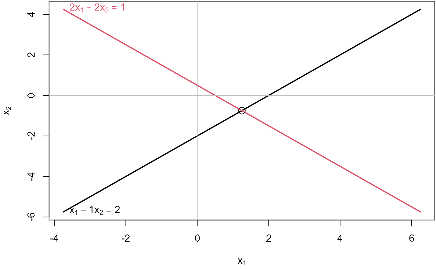

Plot of two consistent equations which plot as lines intersecting in a point

[Solve()](../reference/Solve.html) is a convenience function that shows the solution in a more comprehensible form:

Solve(A, b, fractions = TRUE)

## x1    =   5/4 
##   x2  =  -3/4

Three consistent equations

For three (or more) equations in two unknowns,r(𝐀)≤2r(\mathbf{A}) \le 2, becauser(𝐀)≤min(m,n)r(\mathbf{A}) \le \min(m,n). The equations will be consistent if r(𝐀)=r(𝐀|𝐛)r(\mathbf{A}) = r(\mathbf{A | b}). This means that whatever linear relations exist among the rows of𝐀\mathbf{A}are the same as those among the elements of𝐛\mathbf{b}.

Geometrically, this means that all three lines intersect in a point.

A <- matrix(c(1,2,3, -1, 2, 1), 3, 2)
b <- c(2,1,3)
showEqn(A, b)

## 1*x1 - 1*x2  =  2 
## 2*x1 + 2*x2  =  1 
## 3*x1 + 1*x2  =  3

## [1] 2 2

## [1] TRUE

Solve(A, b, fractions=TRUE)       # show solution

## x1    =   5/4 
##   x2  =  -3/4 
##    0  =     0

Plot the equations:

##   x[1] - 1*x[2]  =  2 
## 2*x[1] + 2*x[2]  =  1 
## 3*x[1]   + x[2]  =  3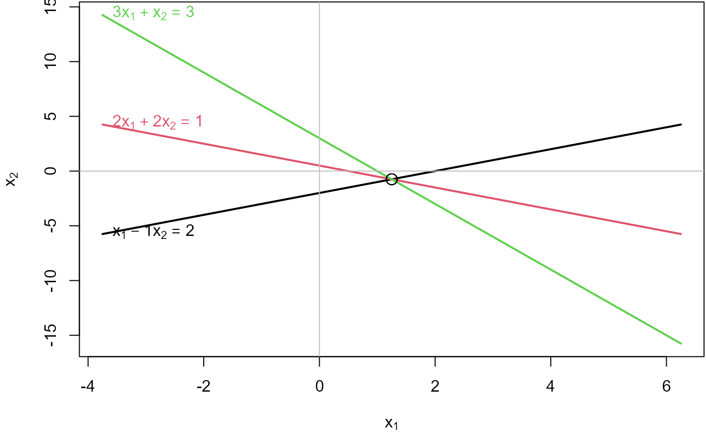

Plot of three consistent equations which plot as three lines intersecting in a point

Three inconsistent equations

Three equations in two unknowns are inconsistent whenr(𝐀)<r(𝐀|𝐛)r(\mathbf{A}) < r(\mathbf{A | b}).

A <- matrix(c(1,2,3, -1, 2, 1), 3, 2)
b <- c(2,1,6)
showEqn(A, b)

## 1*x1 - 1*x2  =  2 
## 2*x1 + 2*x2  =  1 
## 3*x1 + 1*x2  =  6

## [1] 2 3

## [1] "Mean relative difference: 0.5"

You can see this in the result of reducing𝐀|𝐛\mathbf{A} | \mathbf{b}to echelon form, where the last row indicates the inconsistency because it represents the equation0x1+0x2=−30 x_1 + 0 x_2 = -3.

##      [,1] [,2]  [,3]
## [1,]    1    0  2.75
## [2,]    0    1 -2.25
## [3,]    0    0 -3.00

[Solve()](../reference/Solve.html) shows this more explicitly, using fractions where possible:

Solve(A, b, fractions=TRUE)

## x1    =  11/4 
##   x2  =  -9/4 
##    0  =    -3

An approximate solution is sometimes available using a generalized inverse. This gives𝐱=(2,−1)\mathbf{x} = (2, -1)as a best close solution.

##      [,1]
## [1,]    2
## [2,]   -1

Plot the equations. You can see that each pair of equations has a solution, but all three do not have a common, consistent solution.

##   x[1] - 1*x[2]  =  2 
## 2*x[1] + 2*x[2]  =  1 
## 3*x[1]   + x[2]  =  6

# add the ginv() solution
points(x[1], x[2], pch=15)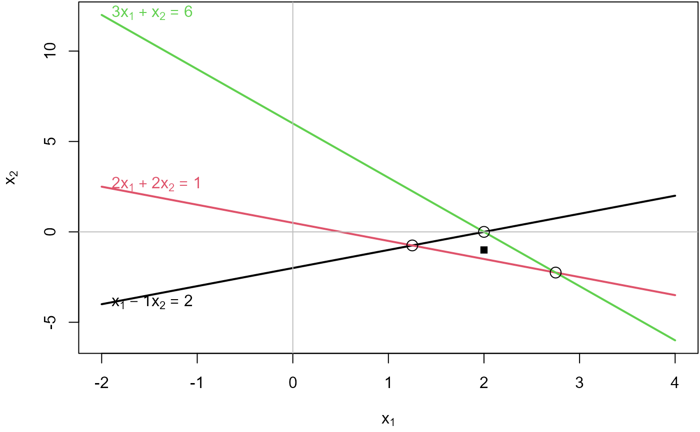

Plot of the lines corresponding to three inconsistent equations. They do not all intersect in a point, indicating that there is no common solution.

Equations in three unknowns

Each equation in three unknowns corresponds to a plane in 3D space. The equations have a unique solution if all planes intersect in a point.

Three consistent equations

An example:

A <- matrix(c(2, 1, -1,
             -3, -1, 2,
             -2,  1, 2), 3, 3, byrow=TRUE)
colnames(A) <- paste0('x', 1:3)
b <- c(8, -11, -3)
showEqn(A, b)

##  2*x1 + 1*x2 - 1*x3  =    8 
## -3*x1 - 1*x2 + 2*x3  =  -11 
## -2*x1 + 1*x2 + 2*x3  =   -3

Are the equations consistent?

## [1] 3 3

## [1] TRUE

Solve for𝐱\mathbf{x}.

## x1 x2 x3 
##  2  3 -1

Other ways of solving:

##    [,1]
## x1    2
## x2    3
## x3   -1

##      [,1]
## [1,]    2
## [2,]    3
## [3,]   -1

Yet another way to see the solution is to reduce𝐀|𝐛\mathbf{A | b}to echelon form. The result of this is the matrix[𝐈|𝐀−𝟏𝐛][\mathbf{I \quad | \quad A^{-1}b}], with the solution in the last column.

##      x1 x2 x3   
## [1,]  1  0  0  2
## [2,]  0  1  0  3
## [3,]  0  0  1 -1

`echelon() can be asked to show the steps, as the row operations necessary to reduce𝐗\mathbf{X}to the identity matrix𝐈\mathbf{I}.

echelon(A, b, verbose=TRUE, fractions=TRUE)

## 
## Initial matrix:

##      x1  x2  x3     
## [1,]   2   1  -1   8
## [2,]  -3  -1   2 -11
## [3,]  -2   1   2  -3
## 
## row: 1 
## 
##  exchange rows 1 and 2

##      x1  x2  x3     
## [1,]  -3  -1   2 -11
## [2,]   2   1  -1   8
## [3,]  -2   1   2  -3
## 
##  multiply row 1 by -1/3

##      x1   x2   x3       
## [1,]    1  1/3 -2/3 11/3
## [2,]    2    1   -1    8
## [3,]   -2    1    2   -3
## 
##  multiply row 1 by 2 and subtract from row 2

##      x1   x2   x3       
## [1,]    1  1/3 -2/3 11/3
## [2,]    0  1/3  1/3  2/3
## [3,]   -2    1    2   -3
## 
##  multiply row 1 by 2 and add to row 3

##      x1   x2   x3       
## [1,]    1  1/3 -2/3 11/3
## [2,]    0  1/3  1/3  2/3
## [3,]    0  5/3  2/3 13/3
## 
## row: 2 
## 
##  exchange rows 2 and 3

##      x1   x2   x3       
## [1,]    1  1/3 -2/3 11/3
## [2,]    0  5/3  2/3 13/3
## [3,]    0  1/3  1/3  2/3
## 
##  multiply row 2 by 3/5

##      x1   x2   x3       
## [1,]    1  1/3 -2/3 11/3
## [2,]    0    1  2/5 13/5
## [3,]    0  1/3  1/3  2/3
## 
##  multiply row 2 by 1/3 and subtract from row 1

##      x1   x2   x3       
## [1,]    1    0 -4/5 14/5
## [2,]    0    1  2/5 13/5
## [3,]    0  1/3  1/3  2/3
## 
##  multiply row 2 by 1/3 and subtract from row 3

##      x1   x2   x3       
## [1,]    1    0 -4/5 14/5
## [2,]    0    1  2/5 13/5
## [3,]    0    0  1/5 -1/5
## 
## row: 3 
## 
##  multiply row 3 by 5

##      x1   x2   x3       
## [1,]    1    0 -4/5 14/5
## [2,]    0    1  2/5 13/5
## [3,]    0    0    1   -1
## 
##  multiply row 3 by 4/5 and add to row 1

##      x1   x2   x3       
## [1,]    1    0    0    2
## [2,]    0    1  2/5 13/5
## [3,]    0    0    1   -1
## 
##  multiply row 3 by 2/5 and subtract from row 2

##      x1 x2 x3   
## [1,]  1  0  0  2
## [2,]  0  1  0  3
## [3,]  0  0  1 -1

Now, let’s plot them.

[plotEqn3d()](../reference/plotEqn3d.html) uses rgl for 3D graphics. If you rotate the figure, you’ll see an orientation where all three planes intersect at the solution point,𝐱=(2,3,−1)\mathbf{x} = (2, 3, -1)

Three inconsistent equations

A <- matrix(c(1,  3, 1,
              1, -2, -2,
              2,  1, -1), 3, 3, byrow=TRUE)
colnames(A) <- paste0('x', 1:3)
b <- c(2, 3, 6)
showEqn(A, b)

## 1*x1 + 3*x2 + 1*x3  =  2 
## 1*x1 - 2*x2 - 2*x3  =  3 
## 2*x1 + 1*x2 - 1*x3  =  6

Are the equations consistent? No.

## [1] 2 3

## [1] "Mean relative difference: 0.5"