11. Vector Spaces of Least Squares and Linear Equations (original) (raw)

This vignette illustrates the relationship between simple linear regression via least squares, in the familiar data space of(x,y)(x, y)and an equivalent representation by means of linear equations for the observations in the less familiarβ\betaspace of the model parameters in the modelyi=β0+β1xi+eiy_i = \beta_0 + \beta_1 x_i + e_i.

In data space, we probably all know that the least squares solution can be visualized as a line with interceptb0≡β0̂b_0 \equiv \widehat{\beta_0}and slopeb1≡β1̂b_1 \equiv \widehat{\beta_1}. But inβ=(β0,β1)\beta = (\beta_0, \beta_1)space, the same solution is the point,(b0,b1)(b_0, b_1).

There is such a pleasing duality here:

A line in data space corresponds to a point in beta space
A point in data space corresponds to a line in beta space

But wait, there’s one more space: observation space, the _n_-dimensional space for n observations. These ideas have a modern history that goes back to Dempster (1969). It was developed in the context of linear models by Fox (1984) and Monette (1990). Some of these geometric relations are explored in a wider context in Friendly et al. (2013).

Data space

We start with a simple linear regression problem, shown indata space.

x <- c(1, 1, -1, -1)
y <- 1:4

Fit the linear model, y ~ x. The intercept isb0 = 2.5 and the slope is b1 = -1.

(mod <- lm(y ~ x))
## 
## Call:
## lm(formula = y ~ x)
## 
## Coefficients:
## (Intercept)            x  
##         2.5         -1.0

Plot the data and the least squares line.

A plot showing 4 points in data space and the linear regression line

Linear equation (β\beta) space

This problem can be represented by the matrix equation,𝐲=[𝟏,𝐱]𝐛+𝐞=𝐗𝐛+𝐞\mathbf{y} = [\mathbf{1}, \mathbf{x}] \mathbf{b} + \mathbf{e} = \mathbf{X} \mathbf{b} + \mathbf{e}.

X <- cbind(1, x)
printMatEqn(y, "=", X, "*", vec(c("b0", "b1")), "+", vec(paste0("e", 1:4)))
##  y         X                  
##  1  =   1  1  *   b0   +   e1 
##  2      1  1      b1       e2 
##  3      1 -1               e3 
##  4      1 -1               e4

Each equation is of the formyi=b0+b1xi+eiy_i = b_0 + b_1 x_i + e_i. The least squares solution minimizes∑ei2\sum e_i^2.

We can also describe this a representing four equations in two unknowns, c("b0", "b1").

showEqn(X, y, vars=c("b0", "b1"), simplify=TRUE)
## b0   + b1  =  1 
## b0   + b1  =  2 
## b0 - 1*b1  =  3 
## b0 - 1*b1  =  4

Each equation corresponds to a line in(b0,b1)(b_0, b_1)space. Let’s plot them. plotEqn draws a point at the intersection of each pair of lines — a solution for that pair of observations.

plotEqn(X, y, vars=c("b0", "b1"), xlim=c(-2, 4))
## b0   + b1  =  1 
## b0   + b1  =  2 
## b0 - 1*b1  =  3 
## b0 - 1*b1  =  4

Each point in data space corresponds to a line in “beta” space. The figure shows the four lines corresponding to the points in the previous figure.

In this space, not all observation equations can be satisfied simultaneously, but a best approximate solution can be represented in this space by the coefficients of the linear modely=Xβy = X \beta, where the intercept is already included as the first column inXX.

plotEqn(X, y, vars=c("b0", "b1"), xlim=c(-2, 4))
## b0   + b1  =  1 
## b0   + b1  =  2 
## b0 - 1*b1  =  3 
## b0 - 1*b1  =  4
solution <- lm( y ~ 0 + X)
loc <- coef(solution)
points(x=loc[1], y=loc[2], pch=16, cex=1.5)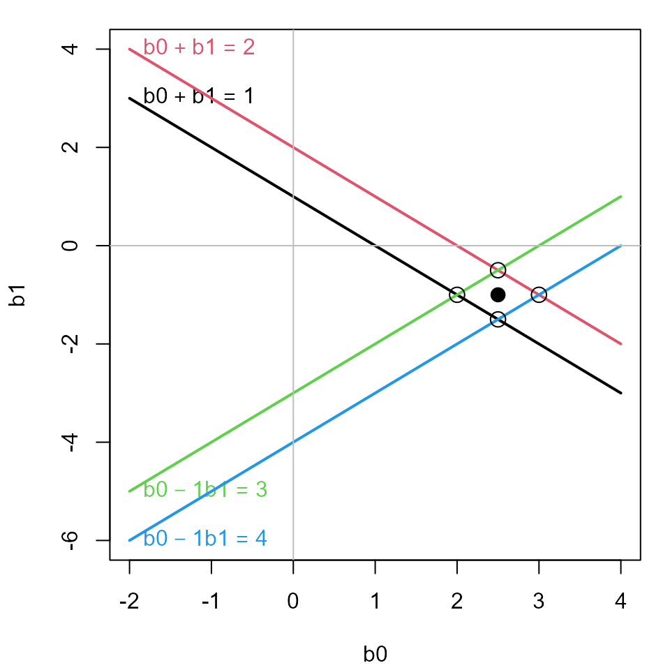

The same as the previous plot of lines, but adding the point (b0, b1) that corresponds to the least squares solution

The LS solution is shown by the black point, corresponding to(b0,b1)=(2.5,−1)(b_0, b_1) = (2.5, -1).

Observation space

There is also a third vector space, one where the coordinate axes refer to the observations,i:ni:n, with data(yi,xi0,xi1,...)(y_i, x_{i0}, x_{i1}, ...). Thenn-length vectors in this space relate to the variables y and predictors x1, x2 … . Here,x0 is the unit vector, J(n), corresponding to the intercept in a model. Fornnobservations, this space hasnndimensions.

In the case of simple linear regression, the fitted values,𝐲̂\widehat{\mathbf{y}}correspond to the projection of𝐲\mathbf{y}on the plane spanned by𝐱𝟎,𝐱𝟏\mathbf{x_0}, \mathbf{x_1}, or yhat <- Proj(y, c(bind(x0, x1))).

In this space, the vector of residuals,𝐞\mathbf{e}is the orthogonal complement of𝐲̂\widehat{\mathbf{y}}, i.e.,𝐲̂⊥𝐞\widehat{\mathbf{y}} \perp \mathbf{e}. Another geometrical description is that the residual vector is the normal vector to the plane.

This space corresponds to the matrix algebra representation of linear regression,

𝐲=𝐗𝐛̂+𝐞=𝐲̂+𝐞\mathbf{y} = \mathbf{X} \widehat{\mathbf{b}} + \mathbf{e} = \widehat{\mathbf{y}} + \mathbf{e} In fact, the least squares solution can be derived purely from the requirement that the vector𝐲̂\widehat{\mathbf{y}}is orthogonal to the vector of residuals,𝐞\mathbf{e}, i.e.,𝐲̂′𝐞=0\widehat{\mathbf{y}}' \mathbf{e} = 0. (The margins of this vignette are too small to give the proof of this assertion.)

Observation space can be illustrated in the vector diagram developed below, but only inn=3n=3dimensional space, for an actual data problem. Here, we createx0, x1 and y for a simple example.

O  <- c(0, 0, 0)    # origin
x0 <- J(3)          # intercept
x1 <- c(0, 1, -1)   # x
y  <- c(1, 1, 4)    # y
y <-  2 * y / floor(len(y))  # make length more convenient for 3D plot

This implies the following linear equations, ignoring residuals.

X <- cbind(x0, x1)      # make a matrix
showEqn(X, y, vars=colnames(X), simplify=TRUE)
## x0         =  0.5 
## x0   + x1  =  0.5 
## x0 - 1*x1  =    2

To display this in observation space,

First create a basic 3D plot showing the coordinate axes.
Then, use [vectors3d()](../reference/vectors3d.html) to draw the vectorsx0, x1 and y.
The plane spanned by x0, and x1 can be specified as as the normal vector orthogonal to both, using the new[matlib::xprod()](../reference/xprod.html) function.
Finally, we use [Proj()](../reference/Proj.html) to find the projection ofy on this plane.

win <- rgl::open3d()
# (1) draw observation axes
E <- diag(3)
rownames(E) <- c("1", "2", "3")
vectors3d(E, lwd=2, color="blue")

# (2) draw variable vectors
vectors3d(t(X), lwd=2, headlength=0.07)
vectors3d(y, labels=c("", "y"), color="red", lwd=3, headlength=0.07)

# (3) draw the plane spanned by x0, x1 
normal <- xprod(x0, x1)
rgl::planes3d(normal, col="turquoise", alpha=0.2)

# (4) draw projection of y on X
py <-  Proj(y, X)
rgl::segments3d(rbind( y, py))       # draw y to plane
rgl::segments3d(rbind( O, py))       # origin to py in the plane
corner( O, py, y, d=0.15)            # show it's a right angle
arc(y, O, py, d=0.2, color="red")

This plot is interactive in the HTML version. Use the mouse wheel to expand/contract the plot. Drag it to rotate to a different view.

You can also spin the plot around it’s any axis or create a movie, but that isn’t done in this vignette.

For comparison, we can also show the least squares solution in data orβ\betaspace. Here it is in linear equation (β\beta) space.

X <- cbind(x0, x1)
plotEqn(X, y, vars=c("b0", "b1"), xlim=c(-2, 4))
## b0         =  0.5 
## b0   + b1  =  0.5 
## b0 - 1*b1  =    2
solution <- lm( y ~ 0 + X)
loc <- coef(solution)
points(x=loc[1], y=loc[2], pch=16, cex=1.5)
abline(v=loc[1], lty=2)
abline(h=loc[2], lty=2)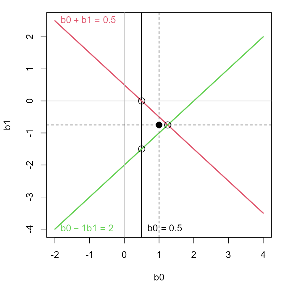

The least squares solution for three points shown in beta space

References

Dempster, A. P. (1969). Elements of Continuous Multivariate Analysis, Addison-Wesley,

Fox, J. (1984). Linear Statistical Models and Related Methods. NY: John Wiley and Sons.

Friendly, M.; Monette, G. & Fox, J. (2013). Elliptical Insights: Understanding Statistical Methods Through Elliptical Geometry Statistical Science, 28, 1-39.

Monette, G. (1990). “Geometry of Multiple Regression and Interactive 3-D Graphics” In: Fox, J. & Long, S. (Eds.) Modern Methods of Data Analysis, SAGE Publications, 209-256