Nanopore R9 rapid run data release · Loman Labs (original) (raw)
30 Jul 2016
R9 data
A long promised addition to the nanopore sequencing repertoire is the rapid sequencing kit. This kit significantly reduces the effort required to make a sequencing library - down from 2-3 hours to a few minutes. We’ve actually played with this kit several times before, once very early on in the MAP (I think using R7 chemistry as long ago as July 2014). More recently, Matt Loose and I tried it out in a hotel room before a famous genomics conference in February of this year. We can both vouch for how easy it is to use - no specialist equipment is required other than pipettes and a source of heat to neutralise the transposase after a short incubation at room temperature. The recommended starting DNA input is 500ng. In our hotel room we used a freshly brewed cup of coffee which provided the required 70 degrees.
The #agbt16 secret sequencing lounge is open ;) pic.twitter.com/iIYqNI5MUD
— Nick Loman (@pathogenomenick) February 10, 2016
However, until recently this kit was really mainly a curiosity rather than a serious proposition because it only produces so-called “1D” data. To remind you, 1D data is when only the template strand of the double-stranded molecule is read. With the 1D kit because there is no hairpin ligation the complement strand does not pass through the pore.
And for R7.3 data this was a significant drawback: sequence accuracy on the template strand is in the low 70s, accuracy-wise, which makes basic tasks like de novo assembly and variant calling computationally very difficult (although probably not impossible, and assemblers like Canu can cope, with a bit of tweaking). It also makes polishing extremely slow.
The release a few months back of the R9 chemistry has changed the game – it’s a game-changer! – and suddenly made 1D reads very usable. This is ascribed to the more discriminatory read head of the CsgG pore employed, where fewer nucleotides in the pore abrogate the flow of ions across the membrane. The spread of electrical current levels is about twice as wide as seen in R7. However it is hard to know exactly how much of the improved accuracy is caused by the pore as this coincided with the introduction of a new style of basecaller that employs ‘deep learning’ (technically a recurrent neural network) rather than the Hidden Markov Model of before. A third change is the introduction of ‘fast mode’, currently running at 250 bases / second, or four times the translocation speed employed with the R7 chemistry. Because all these changes were introduced at once, it is hard to know the relative contribution of each. However, our early access experiences with R7.3 demonstrated that ‘fast mode’ did not seem to have a significant detrimental effect on quality. In fact, the theory is it may improve handling of long homopolymeric tracts by introducing more signal into the ‘dwell’ times.
Other changes: Notably, the sequencing files now record raw current sample data (at 5kHz) by default, and the previous process of linearising the signal into ‘events’ is now performed by the cloud base caller Metrichor rather than MinKNOW on the laptop. Excitingly there are now three local basecallers available - one is built into MinKNOW 1.0.0 (the next release). There is also a separate download called nanonet (available to MAPpers). We tried out nanonet during the ZiBRA bus trip and it worked well, albeit it could not quite keep up with data generation on a standard laptop. Jared Simpson and Matei David also have an open source basecaller called nanocall.
We’ve done two runs of this protocol. The first was on a flowcell that was delivered, erroneously frozen for 36 hours at -10 degrees in our Stores, and then left at room temperature for a week or so (we’d assumed it was completely knackered). We thought we’d just try it out for fun and to our surprise it actually generated a decent yield of data, around 600mb. Data here is from a second flowcell that was correctly stored at fridge temperature.
The final new thing here is that this is a SpotON flowcell; which means the total volume loaded onto the flowcell is halved, and you in fact ‘drip, drip’ the library straight onto the flowcell surface via a small hole that is protected by a plastic clip. What difference this makes to performance is currently unknown:
Freaky new minion loading technique straight on to the flowcell - pic.twitter.com/imEIBrvNrO
— Nick Loman (@pathogenomenick) July 28, 2016
The results from the better flowcell are presented here with links to data at the bottom:
E. coli stats
stats
| Type | Total Reads | Base Pairs | Mean | Median | Min | Max | N25 | N50 | N75 |
|---|---|---|---|---|---|---|---|---|---|
| pass:template | 164472 | 1.48Gb | 9009 | 5944 | 117 | 131969 | 25244 | 14891 | 8074 |
| fail:template | 74465 | 467Mb | 6271 | 3544 | 5 | 328471 | 21903 | 12033 | 6047 |
This is the highest yielding flowcell we’ve ever had, with just shy of 2Gb of base called sequence, and 1.48Gb in the pass bin. Over 99% of the reads map to the reference, meaning the goodput is equivalent to the output.

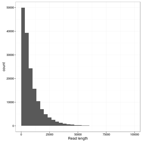
The transpososome method gives a very different size distribution to the Gaussian distribution expected with the traditional Covaris G-tube fragmentation. There are more shorter reads, but the N50 is improved to nearly 15kb (from around 8kb). The maximum length read in this dataset is 131kb and aligns completely to the reference genome at 85% identity.

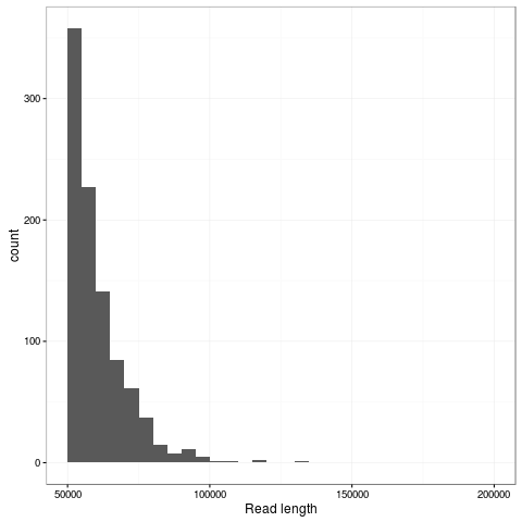
Zooming into this plot it is obvious there are plenty of super long reads - 953 of the passing reads are greater than 50kb comprising 57.5Mb of sequence.

Gratifyingly the data gives a single contig assembly with miniasm and Canu without any custom parameterisation. We’ll pass it over to Jared to see what kind of consensus accuracy he can get out of nanopolish which now has alpha support for R9 data.

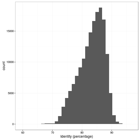
The 1D accuracy is a quantum leap from previous pores, with mean read accuracy at 83%.
We’ll do more analysis on this dataset and hope to write it up as a manuscript in future, but are releasing the dataset for the community to play with.
Links
E. coli 2D kit data
We’ve also previously generated 2D data and this is available below.
Stats
668Mb of passing 2D data (template+complement) results in 244mb of 2D data.
pass stats
| Type | Total Reads | Base Pairs | Mean | Median | Min | Max | N25 | N50 | N75 |
|---|---|---|---|---|---|---|---|---|---|
| template | 50277 | 328543190 | 6534.66 | 6448 | 9 | 78622 | 11688 | 9063 | 6665 |
| complement | 50277 | 340285012 | 6768.2 | 6427 | 5 | 144661 | 12555 | 9280 | 6732 |
| twodirections | 31858 | 244275647 | 7667.64 | 7603 | 99 | 64218 | 11754 | 9244 | 7135 |
Links
- R9 2D FAST5 files (187.2Gb)
- R9 2D all FASTA, MD5
33cba5312402e14d2eda60296ae99bef
ipython notebook
I have posted up the IPython notebook detailing the commands to reproduce this analysis.
Credits
Josh Quick did the laboratory work and sequencing. We are grateful to John Tyson for supplying his tuning scripts for the 1D R9 run.
Conflict of interests
I have received an honorarium to speak at an Oxford Nanopore meeting, and travel and accommodation to attend London Calling 2015 and 2016. I have ongoing research collaborations with ONT although I am not financially compensated for this and hold no stocks, shares or options. ONT have supplied free-of-charge reagents as part of the MinION Access Programme and also generously supported our infectious disease surveillance projects with reagents.