11.1 Comparison-Based Sorting (original) (raw)

Subsections

• 11.1.1 Merge-Sort
• 11.1.2 Quicksort
• 11.1.3 Heap-sort
• 11.1.4 A Lower-Bound for Comparison-Based Sorting

In this section, we present three sorting algorithms: merge-sort, quicksort, and heap-sort. All these algorithms take an input array and sort the elements of into non-decreasing order in (expected) time. These algorithms are all comparison-based. Their second argument, , is a Comparator that implements the method. These algorithms don't care what type of data is being sorted, the only operation they do on the data is comparisons using the method. Recall, from Section 1.1.4, that returns a negative value if , a positive value if , and zero if .

11.1.1 Merge-Sort

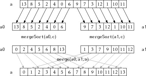
The merge-sort algorithm is a classic example of recursive divide and conquer: If the length of is at most 1, then is already sorted, so we do nothing. Otherwise, we split into two halves, and . We recursively sort and , and then we merge (the now sorted) and to get our fully sorted array :

<T> void mergeSort(T[] a, Comparator<T> c) {
    if (a.length <= 1) return;
    T[] a0 = Arrays.copyOfRange(a, 0, a.length/2);
    T[] a1 = Arrays.copyOfRange(a, a.length/2, a.length);
    mergeSort(a0, c);
    mergeSort(a1, c);
    merge(a0, a1, a, c);
}

An example is shown in Figure 11.1.

**Figure 11.1:**The execution of

Compared to sorting, merging the two sorted arrays and is fairly easy. We add elements to one at a time. If or is empty we add the next elements from the other (non-empty) array. Otherwise, we take the minimum of the next element in and the next element in and add it to :

<T> void merge(T[] a0, T[] a1, T[] a, Comparator<T> c) {
    int i0 = 0, i1 = 0;
    for (int i = 0; i < a.length; i++) {
        if (i0 == a0.length)
            a[i] = a1[i1++];
        else if (i1 == a1.length)
            a[i] = a0[i0++];
        else if (compare(a0[i0], a1[i1]) < 0)
            a[i] = a0[i0++];
        else 
            a[i] = a1[i1++];
    }
}

Notice that the algorithm performs at most comparisons before running out of elements in one of or .

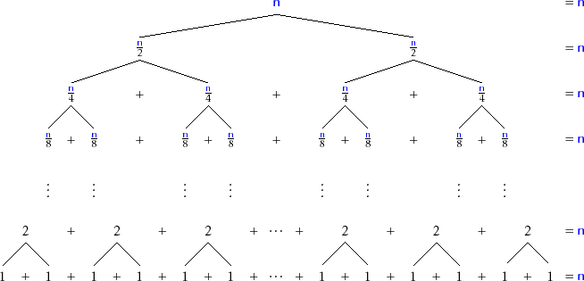
To understand the running-time of merge-sort, it is easiest to think of it in terms of its recursion tree. Suppose for now that is a power of 2, so that , and is an integer. Refer to Figure 11.2. Merge-sort turns the problem of sorting elements into 2 problems, each of sorting elements. These two subproblem are then turned into 2 problems each, for a total of 4 subproblems, each of size . These 4 subproblems become 8 subproblems, each of size , and so on. At the bottom of this process, subproblems, each of size 2, are converted into problems, each of size . 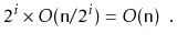For each subproblem of size , the time spent merging and copying data is . Since there are subproblems of size , the total time spent working on problems of size , not counting recursive calls, is

Therefore, the total amount of time taken by merge-sort is

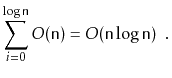
**Figure 11.2:**The merge-sort recursion tree.

The proof of the following theorem is based on the same analysis as above, but has to be a little more careful to deal with the cases where is not a power of 2.

Theorem 11..1 The algorithm runs in time and performs at most comparisons.

Proof. The proof is by induction on

. The base case, in which

, is trivial; when presented with an array of length 0 or 1 the algorithm simply returns without performing any comparisons.

Merging two sorted lists of total length requires at most comparisons. Let denote the maximum number of comparisons performed by on an array of length . If is even, then we apply the inductive hypothesis to the two subproblems and obtain

The case where

is odd is slightly more complicated. For this case, we use two inequalities, that are easy to verify:

	(11.1)

for all and

	(11.2)

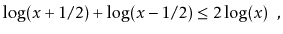
for all . Inequality (11.1) comes from the fact that

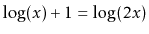while (11.2) follows from the fact that is a concave function. With these tools in hand we have, for odd

,

11.1.2 Quicksort

The quicksort algorithm is another classic divide and conquer algorithm. Unlike merge-sort, which does merging after solving the two subproblems, quicksort does all its work upfront.

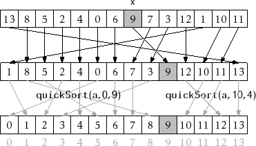
Quicksort is simple to describe: Pick a random pivot element, , from ; partition into the set of elements less than , the set of elements equal to , and the set of elements greater than ; and, finally, recursively sort the first and third sets in this partition. An example is shown in Figure 11.3.

<T> void quickSort(T[] a, Comparator<T> c) {
    quickSort(a, 0, a.length, c);
}
<T> void quickSort(T[] a, int i, int n, Comparator<T> c) {
    if (n <= 1) return;
    T x = a[i + rand.nextInt(n)];
    int p = i-1, j = i, q = i+n;
    // a[i..p]<x,  a[p+1..q-1]??x, a[q..i+n-1]>x 
    while (j < q) {
        int comp = compare(a[j], x);
        if (comp < 0) {       // move to beginning of array
            swap(a, j++, ++p);
        } else if (comp > 0) {
            swap(a, j, --q);  // move to end of array
        } else {
            j++;              // keep in the middle
        }
    }
    // a[i..p]<x,  a[p+1..q-1]=x, a[q..i+n-1]>x 
    quickSort(a, i, p-i+1, c);
    quickSort(a, q, n-(q-i), c);
}

**Figure 11.3:**An example execution of

All of this is done in-place, so that instead of making copies of subarrays being sorted, the method only sorts the subarray . Initially, this method is called as .

At the heart of the quicksort algorithm is the in-place partitioning algorithm. This algorithm, without using any extra space, swaps elements in and computes indices and so that

This partitioning, which is done by the loop in the code, works by iteratively increasing and decreasing while maintaining the first and last of these conditions. At each step, the element at position is either moved to the front, left where it is, or moved to the back. In the first two cases, is incremented, while in the last case, is not incremented since the new element at position has not been processed yet.

Quicksort is very closely related to the random binary search trees studied in Section 7.1. In fact, if the input to quicksort consists of distinct elements, then the quicksort recursion tree is a random binary search tree. To see this, recall that when constructing a random binary search tree the first thing we do is pick a random element and make it the root of the tree. After this, every element will eventually be compared to , with smaller elements going into the left subtree and larger elements going into the right subtree.

In quicksort, we select a random element and immediately compare everything to , putting the smaller elements at the beginning of the array and larger elements at the end of the array. Quicksort then recursively sorts the beginning of the array and the end of the array, while the random binary search tree recursively inserts smaller elements in the left subtree of the root and larger elements in the right subtree of the root.

The above correspondence between random binary search trees and quicksort means that we can translate Lemma 7.1 to a statement about quicksort:

Lemma 11..1 When quicksort is called to sort an array containing the integers , the expected number of times element is compared to a pivot element is at most .

A little summing of harmonic numbers gives us the following theorem about the running time of quicksort:

Theorem 11..2 When quicksort is called to sort an array containing distinct elements, the expected number of comparisons performed is at most .

Proof. Let be the number of comparisons performed by quicksort when sorting

distinct elements. Using Lemma 11.1, we have:

Theorem 11.3 describes the case where the elements being sorted are all distinct. When the input array, , contains duplicate elements, the expected running time of quicksort is no worse, and can be even better; any time a duplicate element is chosen as a pivot, all occurrences of get grouped together and don't take part in either of the two subproblems.

Theorem 11..3 The method runs in expected time and the expected number of comparisons it performs is at most .

11.1.3 Heap-sort

The heap-sort algorithm is another in-place sorting algorithm. Heap-sort uses the binary heaps discussed in Section 10.1. Recall that the BinaryHeap data structure represents a heap using a single array. The heap-sort algorithm converts the input array into a heap and then repeatedly extracts the minimum value.

More specifically, a heap stores elements at array locations with the smallest value stored at the root, . After transforming into a BinaryHeap, the heap-sort algorithm repeatedly swaps and , decrements , and calls so that once again are a valid heap representation. When this process ends (because ) the elements of are stored in decreasing order, so is reversed to obtain the final sorted order.11.1Figure 11.1.3 shows an example of the execution of .

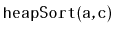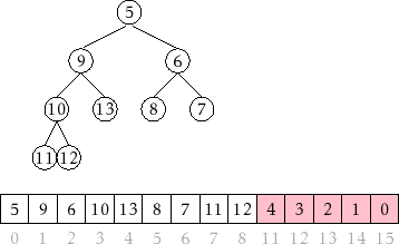
**Figure 11.4:**A snapshot of the execution of . The shaded part of the array is already sorted. The unshaded part is a BinaryHeap. During the next iteration, element will be placed into array location .

<T> void sort(T[] a, Comparator<T> c) {
    BinaryHeap<T> h = new BinaryHeap<T>(a, c);
    while (h.n > 1) {
        h.swap(--h.n, 0);
        h.trickleDown(0);
    }
    Collections.reverse(Arrays.asList(a));
}

A key subroutine in heap sort is the constructor for turning an unsorted array into a heap. It would be easy to do this in time by repeatedly calling the BinaryHeap method, but we can do better by using a bottom-up algorithm. Recall that, in a binary heap, the children of are stored at positions and . This implies that the elements have no children. In other words, each of is a sub-heap of size 1. Now, working backwards, we can call for each . This works, because by the time we call , each of the two children of are the root of a sub-heap so calling makes into the root of its own subheap.

BinaryHeap(T[] a, Comparator<T> c) {
    this.c = c;
    this.a = a;
    n = a.length;
    for (int i = n/2-1; i >= 0; i--) {
        trickleDown(i);
    }
}

The interesting thing about this bottom-up strategy is that it is more efficient than calling times. To see this, notice that, for elements, we do no work at all, for elements, we call on a subheap rooted at and whose height is 1, for elements, we call on a subheap whose height is 2, and so on. Since the work done by is proportional to the height of the sub-heap rooted at , this means that the total work done is at most

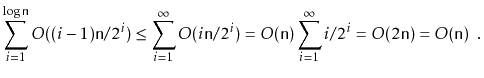
The second-last equality follows by recognizing that the sum is equal, by definition, to the expected number times we toss a coin up to and including the first time the coin comes up as heads and applying Lemma 4.2.

The following theorem describes the performance of .

Theorem 11..4 The method runs in time and performs at most 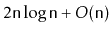comparisons.

Proof. The algorithm runs in 3 steps: (1) Transforming

into a heap, (2) repeatedly extracting the minimum element from

, and (3) reversing the elements in

. We have just argued that step 1 takes

time and performs

comparisons. Step 3 takes

time and performs no comparisons. Step 2 performs

calls to

. The th such call operates on a heap of size

and performs at most

comparisons. Summing this over gives

Adding the number of comparisons performed in each of the three steps completes the proof.

11.1.4 A Lower-Bound for Comparison-Based Sorting

We have now seen three comparison-based sorting algorithms that each run in time. By now, we should be wondering if faster algorithms exist. The short answer to this question is no. If the only operations allowed on the elements of are comparisons then no algorithm can avoid doing roughly comparisons. This is not difficult to prove, but requires a little imagination. Ultimately, it follows from the fact that

(Proving this fact is left as Exercise 11.11.)

We will first focus our attention on deterministic algorithms like merge-sort and heap-sort and on a particular fixed value of . Imagine such an algorithm is being used to sort distinct elements. The key to proving the lower-bound is to observe that, for a deterministic algorithm with a fixed value of , the first pair of elements that are compared is always the same. For example, in , when is even, the first call to is with and the first comparison is between elements and .

Since all input elements are distinct, this first comparison has only two possible outcomes. The second comparison done by the algorithm may depend on the outcome of the first comparison. The third comparison may depend on the results of the first two, and so on. In this way, any deterministic comparison-based sorting algorithm can be viewed as a rooted binary comparison-tree. Each internal node, , of this tree is labelled with a pair of indices and . 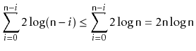If the algorithm proceeds to the left subtree, otherwise it proceeds to the right subtree. Each leaf of this tree is labelled with a permutation of . This permutation represents the permutation that is required to sort if the comparison tree reaches this leaf. That is,

![$\displaystyle \ensuremath{\mathtt{a[w.p[0]]}}<\ensuremath{\mathtt{a[w.p[1]]}}<\cdots<\ensuremath{\mathtt{a[w.p[n-1]]}} \enspace . $](http://opendatastructures.org/versions/edition-0.1e/ods-java/img1437.png)

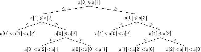
An example of a comparison tree for an array of size is shown in Figure 11.5.

**Figure 11.5:**A comparison tree for sorting an array of length .

The comparison tree for a sorting algorithm tells us everything about the algorithm. It tells us exactly the sequence of comparisons that will be performed for any input array, , having distinct elements and it tells us how the algorithm will reorder to sort it. An immediate consequence of this is that the comparison tree must have at least leaves; if not, then there are two distinct permutations that lead to the same leaf, so the algorithm does not correctly sort at least one of these permutations.

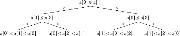
For example, the comparison tree in Figure 11.6 has only leaves. Inspecting this tree, we see that the two input arrays and both lead to the rightmost leaf. On the input this leaf correctly outputs . However, on the input , this node incorrectly outputs . This discussion leads to the primary lower-bound for comparison-based algorithms.

**Figure 11.6:**A comparison tree that does not correctly sort every input permutation.

Theorem 11..5 For any deterministic comparison-based sorting algorithm and any integer , there exists an input array of length such that performs at least 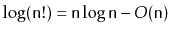comparisons when sorting .

Proof. By the above discussion, the comparison tree defined by

must have at least

leaves. An easy inductive proof shows that any binary tree with leaves has height at least . Therefore, the comparison tree for

has a leaf,

, of depth at least

and there is an input array

that leads to this leaf. The input array

is an input for which

does at least

comparisons.

Theorem 11.5 deals with deterministic algorithms like merge-sort and heap-sort, but doesn't tell us anything about randomized algorithms like quicksort. Could a randomized algorithm beat the lower bound on the number of comparisons? The answer, again, is no. Again, the way to prove it is to think differently about what a randomized algorithm is.

In the following discussion, we will implicitly assume that our decision trees have been ``cleaned up'' in the following way: Any node that can not be reached by some input array is removed. This cleaning up implies that the tree has exactly leaves. It has at least leaves because, otherwise, it could not sort correctly. It has at most leaves since each of the possible permutation of distinct elements follows exactly one root to leaf path in the decision tree.

We can think of a randomized sorting algorithm as a deterministic algorithm that takes two inputs: The input array that should be sorted and a long sequence of random real numbers in the range . The random numbers provide the randomization. When the algorithm wants to toss a coin or make a random choice, it does so by using some element from . For example, to compute the index of the first pivot in quicksort, the algorithm could use the formula .

Now, notice that if we fix to some particular sequence then becomes a deterministic sorting algorithm, , that has an associated comparison tree, . Next, notice that if we select to be a random permutation of , then this is equivalent to selecting a random leaf, , from the leaves of .

Exercise 11.13 asks you to prove that, if we select a random leaf from any binary tree with leaves, then the expected depth of that leaf is at least . Therefore, the expected number of comparisons performed by the (deterministic) algorithm when given an input array containing a random permutation of is at least . Finally, notice that this is true for every choice of , therefore it holds even for . This completes the proof of the lower-bound for randomized algorithms.

Theorem 11..6 For any (deterministic or randomized) comparison-based sorting algorithm and any integer , the expected number of comparisons done by when sorting a random permutation of is at least .

Footnotes

... order.11.1

The algorithm could alternatively redefine the function so that the heap sort algorithm stores the elements directly in ascending order.

opendatastructures.org