Keenan Crane - Monte Carlo Geometry Processing (original) (raw)

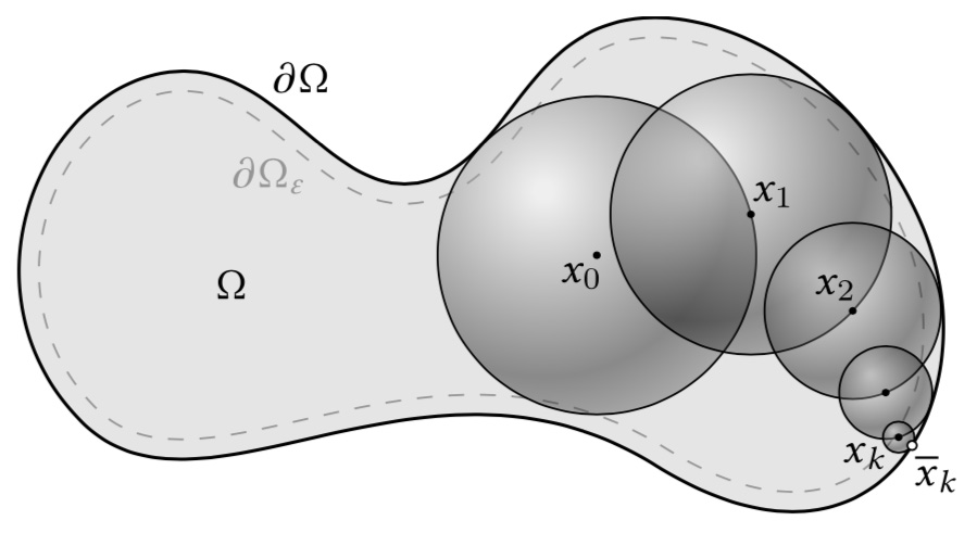
The walk on spheres algorithm repeatedly jumps to a random point on the largest sphere centered at the current point xi , until it gets within ε of the boundary. Since the largest sphere can be determined from a simple closest point query, no spatial discretization is needed.

We can directly solve PDEs on boundary representations not handled by conventional solvers. Left: discontinuous boundary conditions on an implicit surface are captured exactly, whereas FEM or BEM would need a fine mesh to approximate such features. Center: we avoid the daunting challenge of explicit mesh booleans, and can in fact combine heterogeneous representations via constructive solid geometry (CSG). Right: as in rendering, we can compute meaningful solutions for geometry with extremely poor element quality, which degrade gracefully even in the presence of significant noise.

Helmholtz decomposition on a 3D domain. The Monte Carlo approach entirely avoids meshing the domain, setting up matrices, and solving linear systems.

Left: a 3.3M triangle boundary mesh with fine features, from a CT scan of hemisus guineensis (courtesy Blackburn Lab). To visualize the solution to a volumetric PDE, we can significantly reduce cost by computing only a 2D slice of the full 3D solution (right). Inset: fine features are perfectly preserved since we work with the exact input geometry.

Robust meshing methods guarantee success at the cost of geometric accuracy—in this case, completely destroying information about the circulatory and central nervous systems from the previous figure. The Monte Carlo approach exactly preserves these features without hand-tuning of geometric tolerances (nor spending time and memory to precompute a mesh).

Finite element methods exhibit unpredictable performance, since models with simple geometry but poor element quality (left) can confound even robust meshing algorithms (center). The Monte Carlo approach simply needs to build a standard bounding volume hierarchy (right), dramatically reducing the end-to-end cost of solving a PDE.

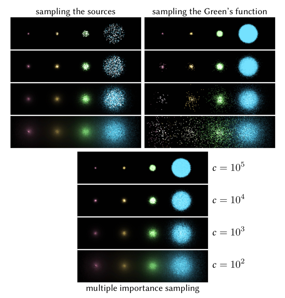
The source term f and Green's function G play the same role as lights and materials in Monte Carlo rendering (resp.); variance can hence be reduced via familiar importance sampling strategies—here we use multiple importance sampling to robustly sample screened Poisson equations for varying coefficients c, with area sources of varying size.

Just as mesh-based methods interpolate solution values at a few sparse points, we can rapidly visualize solutions to PDEs via scattered data interpolation. Here we solve a Laplace problem using either uniform or adaptive sampling and simple MLS interpolation to reduce the sample cost by 100x. Notice that adaptive sampling better resolves the high-frequency boundary conditions.

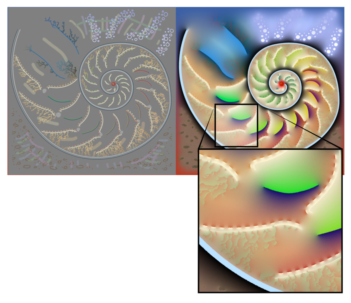
Bézier curves with two-sided boundary conditions plus a source term (left) define a diffusion curve image (right). Monte Carlo allows us to zoom in on a region of interest without computing any kind of global solution; since curves need not be discretized, there is no loss of fidelity.

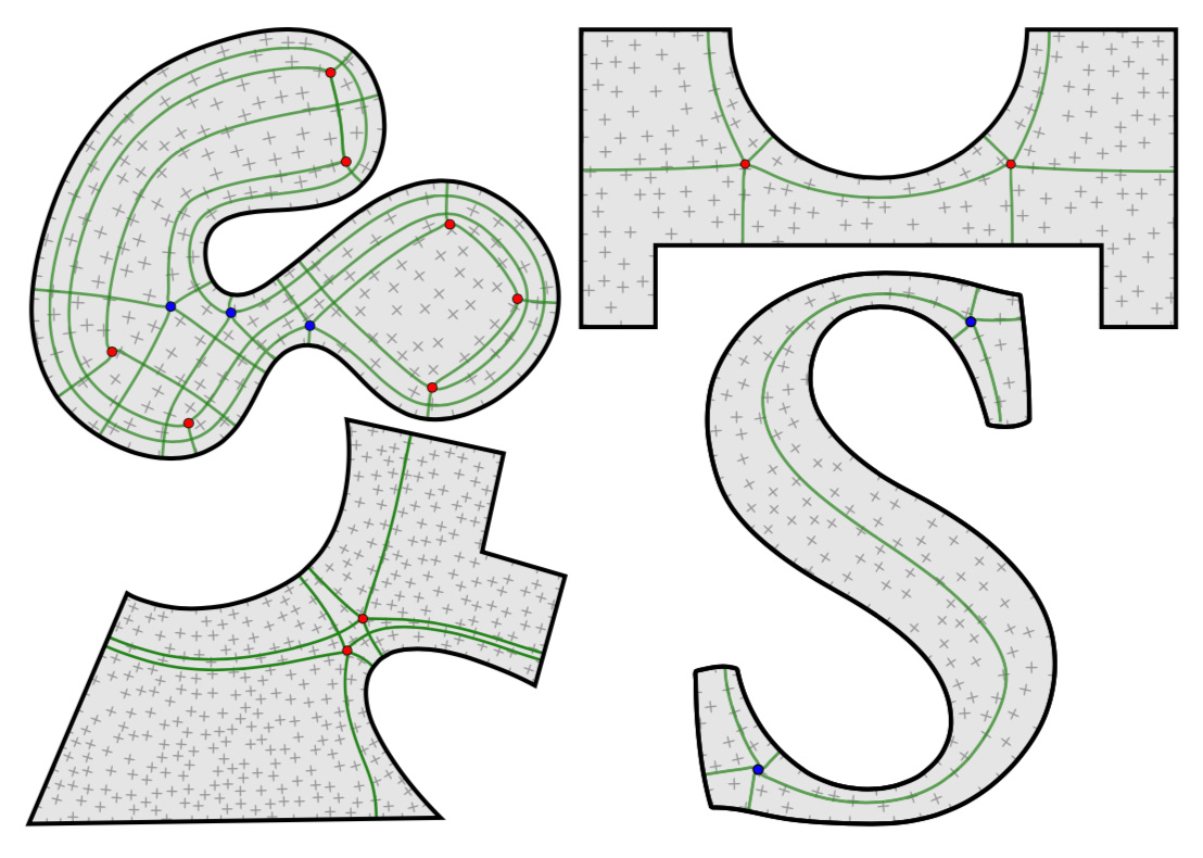
Cross fields and corresponding quad layouts obtained by connecting singular points; no meshes were used at any stage.

We can perform shape deformation by directly editing Bézier curves, including open curves on the shape interior.

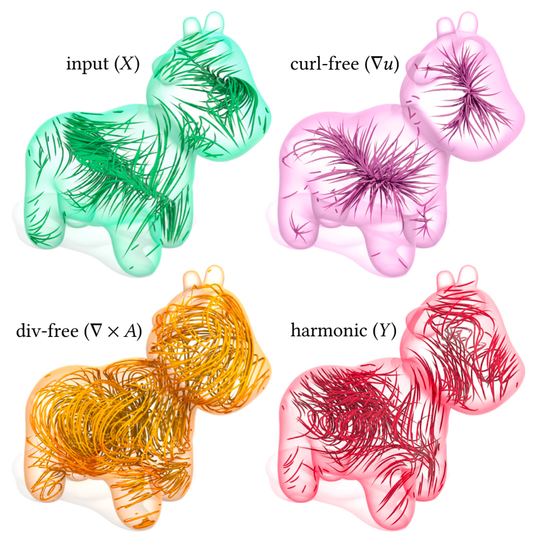
With the Monte Carlo approach, one does not even have to discretize input data. Here we decompose an input vector field X given by a closed-form, analytic expression on a domain with a Bézier boundary curve (top left) into its curl-free, divergence-free, and harmonic components.