Number Precision (original) (raw)

The errors associated with number representation are very similar to quantization errors during ADC. You want to store a continuous range of values; however, you can represent only a finite number of quantized levels. Every time a new number is generated, after a math calculation for example, it must be rounded to the nearest value that can be stored in the format you are using.

As an example, imagine that you allocate 32 bits to store a number. Since there are exactly 232 = 4,294,967,296 different bit patterns possible, you can represent exactly 4,294,967,296 different numbers. Some programming languages allow a variable called a long integer, stored as 32 bits, fixed point, two's complement. This means that the 4,294,967,296 possible bit patterns represent the integers between -2,147,483,648 and 2,147,483,647. In comparison, single precision floating point spreads these 4,294,967,296 bit patterns over the much larger range: -3.4 × 1038 to 3.4 ? 1038.

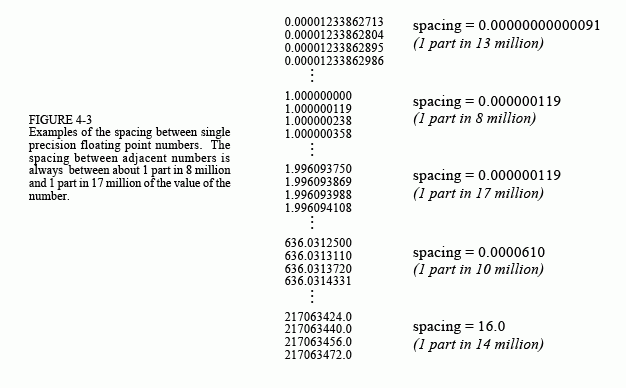
With fixed point variables, the gaps between adjacent numbers are always_exactly one_. In floating point notation, the gaps between adjacent numbers vary over the represented number range. If we randomly pick a floating point number, the gap next to that number is approximately _ten million times smaller_than the number itself (to be exact, 2-24 to 2-23 times the number). This is a key concept of floating point notation: large numbers have large gaps between them, while small numbers have small gaps. Figure 4-3 illustrates this by showing consecutive floating point numbers, and the gaps that separate them.

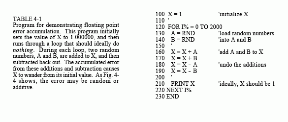
The program in Table 4-1 illustrates how round-off error (quantization error in math calculations) causes problems in DSP. Within the program loop, two random numbers are added to the floating point variable X, and then subtracted back out again. Ideally, this should do nothing. In reality, the round-off error from each of the arithmetic operations causes the value of X to gradually drift away from its initial value. This drift can take one of two forms depending on how the errors add together. If the round-off errors are randomly positive and negative, the value of the variable will randomly increase and decrease. If the errors are predominately of the same sign, the value of the variable will drift away much more rapidly and uniformly.

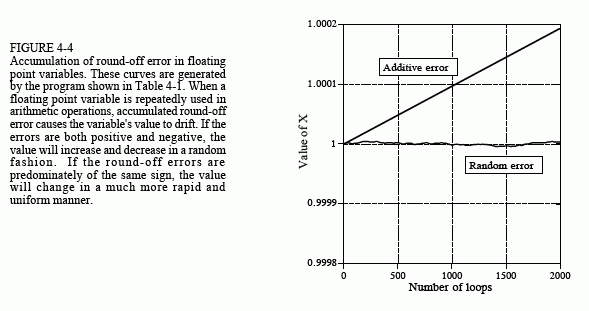
Figure 4-4 shows how the variable, X, in this example program drifts in value. An obvious concern is that additive error is much worse than random error. This is because random errors tend to cancel with each other, while the additive errors simply accumulate. The additive error is roughly equal to the round-off error from a single operation, multiplied by the total number of operations. In comparison, the random error only increases in proportion to the square root of the number of operations. As shown by this example, additive error can be hundreds of times worse than random error for common DSP algorithms.

Unfortunately, it is nearly impossible to control or predict which of these two behaviors a particular algorithm will experience. For example, the program in Table 4-1 generates an additive error. This can be changed to a random error by merely making a slight modification to the numbers being added and subtracted. In particular, the random error curve in Fig. 4-4 was generated by defining: A = EXP(RND) and B = EXP(RND), rather than: A = RND and B = RND. Instead of A and B being randomly distributed numbers between 0 and 1, they become exponentially distributed values between 1 and 2.718. Even this small change is sufficient to toggle the mode of error accumulation.

Since we can't control which way the round-off errors accumulate, keep in mind the worse case scenario. Expect that every single precision number will have an error of about one part in forty million, multiplied by the number of operations it has been through. This is based on the assumption of additive error, and the average error from a single operation being one-quarter of a quantization level. Through the same analysis, every double precision number has an error of about_one part in forty quadrillion, multiplied by the number of operations._

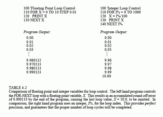
Table 4-2 illustrates a particularly annoying problem of round-off error. Each of the two programs in this table perform the same task: printing 1001 numbers equally spaced between 0 and 10. The left-hand program uses the floating point variable, X, as the loop index. When instructed to execute a loop, the computer begins by setting the index variable to the starting value of the loop (0 in this example). At the end of each loop cycle, the step size (0.01 in the case) is_added_ to the index. A decision is then made: are more loops cycles required, or is the loop completed? The loop ends when the computer finds that the value of the index is greater than the termination value (in this example, 10.0). As shown by the generated output, round-off error in the additions cause the value of X to accumulate a significant discrepancy over the course of the loop. In fact, the accumulated error prevents the execution of the last loop cycle. Instead of_X_ having a value of 10.0 on the last cycle, the error make the last value of _X_equal to 10.000133. Since X is greater than the termination value, the computer thinks its work is done, and the loop prematurely ends. This missing last value is a common bug in many computer programs.

In comparison, the program on the right uses an integer variable, I%, to control the loop. The addition, subtraction, or multiplication of two integers always produces another integer. This means that fixed point notation has absolutely no round-off error with these operations. Integers are ideal for controlling loops, as well as other variables that undergo multiple mathematical operations. The last loop cycle is guaranteed to execute! Unless you have some strong motivation to do otherwise, always use integers for loop indexes and counters.

If you must use a floating point variable as a loop index, try to use fractions that are a power of two (such as: 1/2, 1/4, 3/8, 27/16), instead of a power of ten (such as: 0.1, 0.6, 1.4, 2.3, etc.). For instance, it would be better to use: FOR X = 1 TO 10 STEP 0.125, rather than: FOR X = 1 to 10 STEP 0.1. This allows the index to always have an exact binary representation, thereby reducing round-off error. For example, the decimal number: 1.125, can be represented exactly in binary notation: 1.001000000000000000000000×20. In comparison, the decimal number: 1.1, falls between two floating point numbers: 1.0999999046 and 1.1000000238 (in binary these numbers are: 1.00011001100110011001100?20 and 1.00011001100110011001101?20). This results in an inherent error each time 1.1 is encountered in a program.

A useful fact to remember: single precision floating point has an exact binary representation for every whole number between +16.8 million (to be exact, ±224). Above this value, the gaps between the levels are larger than one, causing some whole number values to be missed. This allows floating point whole numbers (between ±16.8 million) to be added, subtracted and multiplied, with no round-off error.