Classification and diagnostic prediction of cancers using gene expression profiling and artificial neural networks (original) (raw)
. Author manuscript; available in PMC: 2005 Nov 10.
Published in final edited form as: Nat Med. 2001 Jun;7(6):673–679. doi: 10.1038/89044
Abstract
The purpose of this study was to develop a method of classifying cancers to specific diagnostic categories based on their gene expression signatures using artificial neural networks (ANNs). We trained the ANNs using the small, round blue-cell tumors (SRBCTs) as a model. These cancers belong to four distinct diagnostic categories and often present diagnostic dilemmas in clinical practice. The ANNs correctly classified all samples and identified the genes most relevant to the classification. Expression of several of these genes has been reported in SRBCTs, but most have not been associated with these cancers. To test the ability of the trained ANN models to recognize SRBCTs, we analyzed additional blinded samples that were not previously used for the training procedure, and correctly classified them in all cases. This study demonstrates the potential applications of these methods for tumor diagnosis and the identification of candidate targets for therapy.
The small, round blue cell tumors (SRBCTs) of childhood, which include neuroblastoma (NB), rhabdomyosarcoma (RMS), non-Hodgkin lymphoma (NHL) and the Ewing family of tumors (EWS), are so named because of their similar appearance on routine histology1. However, accurate diagnosis of SRBCTs is essential because the treatment options, responses to therapy and prognoses vary widely depending on the diagnosis. As their name implies, these cancers are difficult to distinguish by light microscopy, and currently no single test can precisely distinguish these cancers. In clinical practice, several techniques are used for diagnosis, including immunohistochemistry2, cytogenetics, interphase fluorescence in situ hybridization3 and reverse transcription (RT)-PCR (ref. 4). Immunohistochemistry allows the detection of protein expression, but it can only examine one protein at a time. Molecular techniques such as RT-PCR are used increasingly for diagnostic confirmation following the discovery of tumor-specific translocations such as EWS-FLI1; t(11;22)(q24;q12) in EWS, and the PAX3-FKHR; t(2;13)(q35;q14) in alveolar rhabdomyosarcoma1 (ARMS). However, molecular markers do not always provide a definitive diagnosis, as on occasion there is failure to detect the classical translocations, due to either technical difficulties or the presence of variant translocations.
Gene-expression profiling using cDNA microarrays permits a simultaneous analysis of multiple markers, and has been used to categorize cancers into subgroups5–8. However, despite the many statistical techniques to analyze gene-expression data, none so far has been rigorously tested for their ability to accurately distinguish cancers belonging to several diagnostic categories.
Artificial neural networks (ANNs) are computer-based algorithms which are modeled on the structure and behavior of neurons in the human brain and can be trained to recognize and categorize complex patterns9. Pattern recognition is achieved by adjusting parameters of the ANN by a process of error minimization through learning from experience. They can be calibrated using any type of input data, such as gene-expression levels generated by cDNA microarrays, and the output can be grouped into any given number of categories. ANNs have been recently applied to clinical problems such as diagnosing myocardial infarcts10 and arrhythmias from electrocardiograms11 and interpreting radiographs and magnetic resonance images12,13. Here we applied ANNs to decipher gene-expression signatures of SRBCTs and used them for diagnostic classification.
Calibration and validation of the ANN models
To calibrate ANN models to recognize cancers in each of the four SRBCT categories, we used gene-expression data from cDNA microarrays containing 6567 genes. The 63 training samples (see Supplemental Table A) included both tumor biopsy material (13 EWS and 10 RMS) and cell lines (10 EWS, 10 RMS, 12 NB and 8 Burkitt lymphomas (BL; a subset of NHL)). For two samples, ST486 (BL-C2 and C4) and GICAN (NB-C2 and C7), we performed two independent microarray experiments to test the reproducibility of the experiments and these were subsequently treated as separate samples. Filtering for a minimal level of expression reduced the number of genes to 2308 (Fig. 1_a_). Principal component analysis (PCA) further reduced the dimensionality, and we found that using the 10 dominant PCA components per sample as inputs and four outputs (EWS, RMS, NB or BL) produced well-calibrated ANN models. These 10 dominant components contained 63% of the variance in the data matrix. The remaining PCA components contained variance unrelated to separating the four cancers. The three-fold cross-validation procedure (see Methods) produced a total of 3750 ANN models, and the training and validation was successful (Fig. 1_b_). In addition, there was no sign of ‘over-training’ of the models, as would be shown by a rise in the summed square error for the validation set with increasing training iterations or ‘epochs’ (Fig. 1_b_). Using these ANN models, all of the 63 training samples were correctly assigned/classified to their respective categories, having received the highest committee vote (average output) for that category.
Fig. 1.
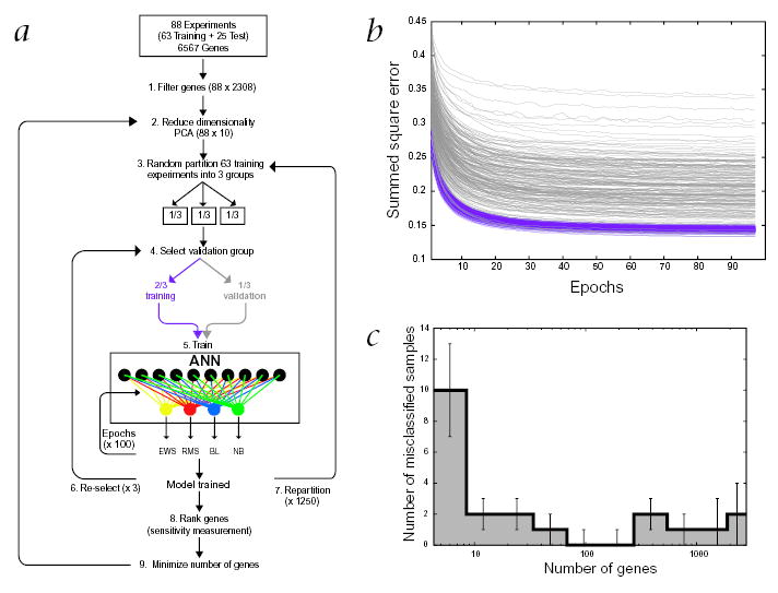
The artificial neural network. a, Schematic illustration of the analysis process. The entire data-set of all 88 experiments was first quality filtered (1) and then the dimensionality was further reduced by principal component analysis (PCA) to 10 PCA projections (2), from the original 6567 expression values. Next, the 25 test experiments were set aside and the 63 training experiments were randomly partitioned into 3 groups (3). One of these groups was reserved for validation and the remaining 2 groups for calibration (4). ANN models were then calibrated using for each sample the 10 PCA values as input and the cancer category as output (5). For each model the calibration was optimized with 100 iterative cycles (epochs). This was repeated using each of the 3 groups for validation (6). The samples were again randomly partitioned and the entire training process repeated (7). For each selection of a validation group one model was calibrated, resulting in a total of 3750 trained models. Once the models were calibrated they were used to rank the genes according to their importance for the classification (8). The entire process (2–7) was repeated using only top ranked genes (9). The 25 test experiments were subsequently classified using all the calibrated models. b, Monitoring the calibration of the models. The average classification error per sample (using a summed square error function) is plotted during the training iterations (epochs) for both the training and the validation samples. A pair of lines, purple (training) and gray (validation), represents one model. The decrease in the classification errors with increasing epochs demonstrates the learning of the models to distinguish these cancers. The results shown are for 200 different models, each corresponding to a random partitioning of the data. All the models performed well for both training and validation as demonstrated by the parallel decrease (with increasing epochs) of the average summed square classification error per sample. In addition, there was no sign of over-training: if the models begin to learn features in the training set, which are not present in the validation set, this would result in an increase in the error for the validation at that point and the curves would no longer remain parallel. c, Minimizing the number of genes. The average number of misclassified samples for all 3750 models is plotted against increasing number of used genes. The misclassifications minimized to zero using the 96 highest ranked genes.
Optimization of genes utilized for classification
We next determined the contribution of each gene to the classification by the ANN models by measuring the sensitivity of the classification to a change in the expression level of each gene, using the 3750 previously calibrated models (see Supplementary Methods). In this way, we ranked the genes according to their significance for the classification. We then determined the classification error rate using increasing numbers of these ranked genes. The classification error rate minimized to 0% at 96 genes (Fig. 1_c_). The 10 dominant PCA components for these 96 genes contained 79% of the variance in the data matrix. Using only these 96 genes, we recalibrated the ANN models (Fig. 1_a_) and again correctly classified all 63 samples (Fig. 2). Moreover, multidimensional scaling (MDS) analysis5 using these 96 genes clearly separated the four cancer types (Fig. 3_a_). The top 96 discriminators represented 93 unique genes (Fig. 3_b_), as IGF2 was represented by three independent clones and MYC by two. Of the 96, 13 were anonymous expressed sequence tags (ESTs); 16 genes were specifically expressed in EWS, 20 in RMS, 15 in NB and 10 in BL. Twelve genes were good discriminators on the basis of lack of expression in BL and variable expression in the other three types. One gene (EST; Clone ID 295985) discriminated EWS from other cancer types by its lack of expression in this cancer. The remainder of the genes was expressed in two of the four cancer types. To our knowledge, of the 61 genes that were specifically expressed in a cancer type, 41 have not been previously reported as associated with these diseases.
Fig. 2.
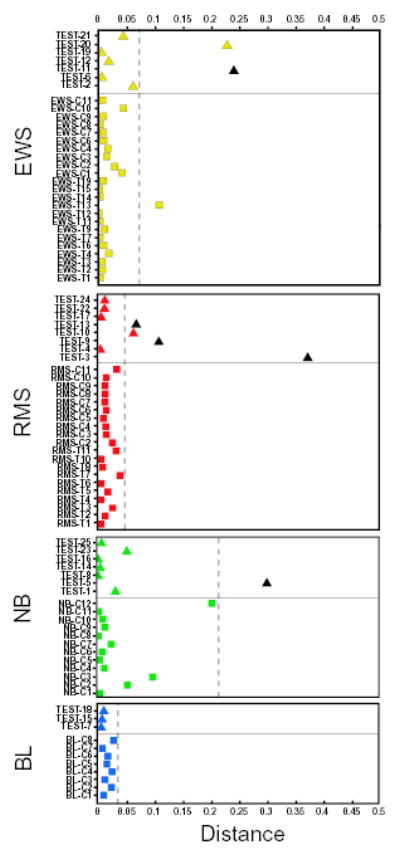
Classification and diagnosis of the samples. A sample is classified to a cancer category according to its highest committee vote (average of all ANN outputs) and placed in the corresponding plot. Plotted, for each sample, is the distance from its committee vote to the ideal vote for that diagnostic category (for example, for EWS, it is EWS = 1, RMS = NB = BL = 0). Thus a perfectly classified sample would be plotted with a distance of zero. Training samples are displayed as squares and test samples as triangles. Non-SRBCT samples are colored black. All SRBCT samples, including the 20 tests, were correctly classified. The distance corresponding to the 95th percentile for the training samples is represented by a dashed line, outside which the diagnosis of a sample is rejected. The diagnosis of all 5 non-SRBCT test samples was rejected since they lie outside their respective dashed lines. Three of the SRBCT samples (EWS-T13, TEST-10 and TEST-20) though correctly classified could not be confidently diagnosed.
Fig. 3.
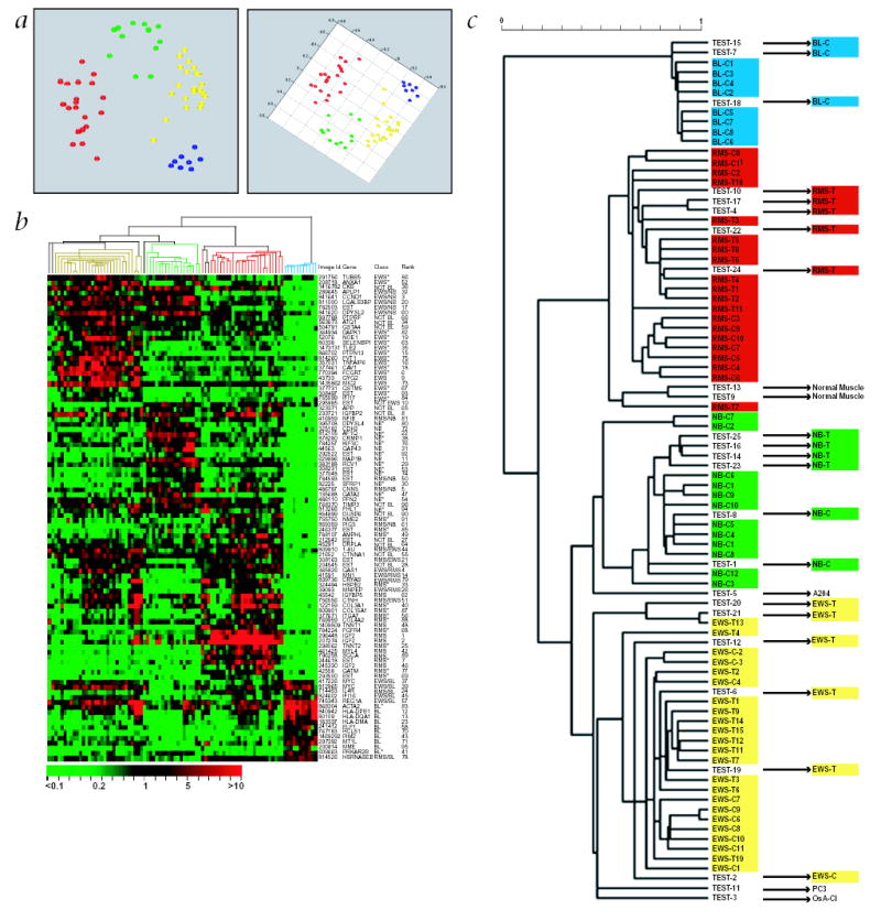
Hierarchical clustering and multidimensional scaling analysis. The top 96 genes as ranked by the ANN models were used for the analysis. a, Multidimensional scaling analysis. Shown here are two projections of the MDS plot of the training samples. EWS are depicted as yellow circles, RMS as red, BL as blue and NB as green. The samples clustered closely according to the 4 different cancer categories. b, Hierarchical clustering of the samples and genes. Each row represents one of the 96 cDNA clones and each column a separate sample. A pseudo-colored representation of the relative red intensity is shown such that a red color indicates high expression and green color low expression, with scale shown below. On the right are the IMAGE id., gene symbol, class in which the gene is highly expressed (see Supplementary Methods), and the ANN rank. *, genes that have not been reported to be associated with these cancers. c, Enlargement of the hierarchical clustering dendrogram of the samples in b. All 63 training and the 20 test SRBCTs correctly clustered within their diagnostic categories. In both cases where two samples were derived from the same cell line, BL-C2 & C4, and NB-C2 and C7, each mapped adjacent to one another in the same cluster. The scale shows the Pearson correlation coefficient used to construct the dendrogram. The Pearson correlation cutoff was 0.54, when the samples clustered into the four diagnostic categories.
Diagnostic classification and hierarchical clustering
We then tested the diagnostic classification capabilities of these ANN models on a set of 25 blinded test samples. A sample is classified to a diagnostic category if it receives the highest vote for that category and because this classifier has only four possible outputs, all samples will be classified to one of the four categories. We therefore established a diagnostic classification method based on a statistical cutoff to enable us to reject a diagnosis of a sample classified to a given category. If a sample falls outside the 95th percentile of the probability distribution of distances between samples and their ideal output (for example, for EWS it is EWS = 1, RMS = NB = BL = 0), its diagnosis is rejected (see Methods).
The test samples contained both tumors (5 EWS, 5 RMS and 4 NB) and cell lines (1 EWS, 2 NB and 3 BL). We also tested the ability of these models to reject a diagnosis on 5 non-SRBCTs (consisting of 2 normal muscle tissues (Tests 9 and 13) and 3 cell lines including an undifferentiated sarcoma (Test 5), osteosarcoma (Test 3) and a prostate carcinoma (Test 11)). Using the 3750 ANN models calibrated with the 96 genes, we correctly classified 100% of the 20 SRBCT tests (Table 1 & Fig. 2) as well as all 63 training samples (see Supplemental Table A). Three of these samples, Test 10, Test 20 and EWS-T13 were correctly assigned to their categories (RMS, EWS and EWS respectively), having received the highest vote for their respective categories. However, their distance from a perfect vote was greater than the expected 95th percentile distance (Fig. 2); therefore, we could not confidently diagnose them by this criterion. All of the five non-SRBCT samples were excluded from any of the four diagnostic categories, since they fell outside the 95th percentiles. Using these criteria for all 88 samples, the sensitivity of the ANN models for diagnostic classification was 93% for EWS, 96% for RMS and 100% for both NB and BL. The specificity was 100% for all four diagnostic categories. Also, hierarchical clustering14 using the 96 genes, identified from the ANN models, correctly clustered all 20 of the test samples (Fig. 3_c_). Moreover, the two pairs of samples that were derived from two cell lines, BL-C2 and C4 (ST486) and NB-C2 and C7 (GICAN), were adjacent to one another in the same cluster.
Table 1.
ANN diagnostic prediction
| ANN committee vote | |||||||||
|---|---|---|---|---|---|---|---|---|---|
| Sample label | EWS | RMS | NB | BL | ANN classification | ANN diagnosis | Histological diagnosis | Source label | Source |
| Test 1 | 0.01 | 0.07 | 0.76 | 0.06 | NB | NB | NB-C | IMR32 | ATCC |
| Test 2 | 0.67 | 0.06 | 0.08 | 0.09 | EWS | EWS | EWS-C | CHOP1 | NCI |
| Test 3 | 0.11 | 0.17 | 0.16 | 0.11 | RMS | - | Osteosarcoma-C | OsA-Cl | ATCC |
| Test 4 | 0.00 | 0.95 | 0.06 | 0.03 | RMS | RMS | ARMS-T | ARMD1 | CHTN |
| Test 5 | 0.11 | 0.11 | 0.25 | 0.10 | NB | - | Sarcoma-C | A204 | ATCC |
| Test 6 | 0.98 | 0.04 | 0.10 | 0.03 | EWS | EWS | EWS-T | 9608P053 | CHTN |
| Test 7 | 0.05 | 0.02 | 0.05 | 0.93 | BL | BL | BL-C | EB1 | ATCC |
| Test 8 | 0.00 | 0.05 | 0.94 | 0.04 | NB | NB | NB-C | SMSSAN | NCI |
| Test 9 | 0.22 | 0.60 | 0.03 | 0.06 | RMS | - | Sk. Muscle | SkM1 | CHTN |
| Test 10 | 0.10 | 0.68 | 0.11 | 0.04 | RMS | - | ERMS-T | ERDM1 | CHTN |
| Test 11 | 0.39 | 0.04 | 0.28 | 0.15 | EWS | - | Prostate Ca.-C | PC3 | ATCC |
| Test 12 | 0.89 | 0.05 | 0.14 | 0.03 | EWS | EWS | EWS-T | SARC67 | CHTN |
| Test 13 | 0.20 | 0.7 | 0.03 | 0.05 | RMS | - | Sk. Muscle | SkM2 | CHTN |
| Test 14 | 0.03 | 0.02 | 0.90 | 0.07 | NB | NB | NB-T | NB3 | DZNSG |
| Test 15 | 0.06 | 0.03 | 0.05 | 0.91 | BL | BL | BL-C | EB2 | ATCC |
| Test 16 | 0.03 | 0.02 | 0.93 | 0.05 | NB | NB | NB-T | NB1 | DZNSG |
| Test 17 | 0.01 | 0.90 | 0.05 | 0.03 | RMS | RMS | ARMS-T | ARMD2 | CHTN |
| Test 18 | 0.06 | 0.04 | 0.04 | 0.88 | BL | BL | BL-C | GA10 | ATCC |
| Test 19 | 0.99 | 0.02 | 0.04 | 0.05 | EWS | EWS | EWS-T | ET3 | CHTN |
| Test 20 | 0.40 | 0.30 | 0.10 | 0.06 | EWS | - | EWS-T | 9903P1339 | CHTN |
| Test 21 | 0.81 | 0.19 | 0.12 | 0.04 | EWS | EWS | EWS-T | ES23 | MSKCC |
| Test 22 | 0.01 | 0.88 | 0.09 | 0.04 | RMS | RMS | ERMS-T | ERMD2 | CHTN |
| Test 23 | 0.07 | 0.08 | 0.70 | 0.06 | NB | NB | NB-T | NB2 | DZNSG |
| Test 24 | 0.05 | 0.87 | 0.06 | 0.03 | RMS | RMS | ERMS-T | RMS4 | MSKCC |
| Test 25 | 0.05 | 0.02 | 0.89 | 0.06 | NB | NB | NB-T | NB4 | DZNSG |
Expression of FGFR4 on SRBCT tissue array
To confirm the effectiveness of the ANN models to identify genes that show preferential high expression in specific cancer types at the protein level, we performed immunohistochemistry on SRBCT tissue arrays for the expression of fibroblast growth factor receptor 4 (FGFR4). This tyrosine kinase receptor is expressed during myogenesis15 but not in adult muscle, and is of interest because of its potential role in tumor growth16 and in prevention of terminal differentiation in muscle17. Moderate to strong cytoplasmic immunostaining for FGFR4 was seen in all 26 RMSs tested (17 alveolar, 9 embryonal). We also observed generally weaker staining in EWS and NHL in agreement with the microarray results, except for one case of anaplastic large cell lymphoma that was strongly positive (data not shown).
Discussion
Tumors are currently diagnosed by histology and immunohistochemistry based on their morphology and protein expression, respectively. However, poorly differentiated cancers can be difficult to diagnose by routine histopathology. In addition, the histological appearance of a tumor cannot reveal the underlying genetic aberrations or biological processes that contribute to the malignant process. Here we developed a method of diagnostic classification of cancers from their gene-expression signatures and identified the genes that contributed to this classification.
We used the SRBCTs of childhood as a model because these cancers occasionally present diagnostic difficulties. For example, Ewing sarcoma is diagnosed by immunohistochemical evidence of MIC2 expression18 and lack of expression of the leukocyte common antigen CD45 (excluding lymphoma), muscle-specific actin or myogenin (excluding RMS)19. However, reliance on detection of MIC2 alone can lead to incorrect diagnosis as MIC2 expression occurs occasionally in other tumor types including RMS and NHL (ref. 1).
Monitoring global gene-expression levels by cDNA microarrays provides an additional tool for elucidating tumor biology as well as the potential for molecular diagnostic classification of cancer5–8,20–22. Currently, classification and clustering tools using gene-expression data have not been rigorously tested for diagnostic classification of more than two categories. Other approaches that share the parametric nature of ANNs and have been utilized to classify gene-expression profiles include Support Vector Machines23. Thus far, these other methods have not been fully explored to extract the genes or features that are most important for the classification performance and which also will be of interest to cancer biologists24.
Here we have approached this problem using ANN-based models. We calibrated ANN models on the expression profiles of 63 SRBCTs of 4 diagnostic categories. Due to the limited amount of training data and the high performance achieved, we limited our analysis to linear (that is, no hidden layers) ANN models. Although other linear methods may perform as well, our method can easily accommodate nonlinear features of expression data if required. To compensate for heterogeneity within the tumor samples (which contain both malignant and stromal cells) and for possible artifacts due to growth of cell lines in tissue culture, we used both tumor samples (n = 23) and cell lines (n = 40). Data from these samples is complementary, because tumor tissue, though complex, provides a gene-expression pattern representative of tumor growth in vivo, while cell lines contain a uniform malignant population without stromal contamination. Despite using only NB cell lines for calibrating the ANN models, all four NB tumors among the test samples were correctly diagnosed with high confidence. This not only demonstrates the high similarity of NB cell lines to the tumors of origin, but also validates the use of cell lines for ANN calibration. The calibrated ANN models accurately classified all 63 training SRBCTs and showed no evidence of over-training, demonstrating the robustness of this technique.
A potential difficulty with ANN-based pattern recognition models is elucidating causal links from the output to the original input data. To solve this problem and to identify the most significant genes, we calculated the sensitivity of the classification to a change in the expression level of each gene. We produced a list of genes ranked by their significance to the classification. Using this list, we established that the top 96 genes reduced the misclassifications to zero, which opens the potential for cost effective fabrication of SRBCT subarrays in diagnostic use. When we tested the ANN models calibrated using the 96 genes on 25 blinded samples, we were able to correctly classify all 20 samples of SRBCTs and reject the 5 non-SRBCTs. This supports the potential use of these methods as an adjunct to routine histological diagnosis.
Although ANN analysis leads to identification of genes specific for a cancer with implications for biology and therapy, a strength of this method is that it does not require genes to be exclusively associated with a single cancer type. This allows for classification based on complex gene-expression patterns. For example, the top 96 discriminating genes included not only those that had high (61) or low levels (12 BL and 1 EWS) of expression in one particular cancer, but also genes that were differentially expressed in two diagnostic categories as compared to the remaining two. Of the 16 genes highly expressed only in EWS, two (MIC2 and GYG2) have been previously described18,25. MIC2 immunostaining is currently used to diagnose EWS; however we find that although MIC2 detects EWS with high sensitivity, it alone cannot be used to discriminate EWS as it was also expressed in several RMSs.
Our method identifies genes related to tumor histogenesis, but includes genes that may not normally be expressed in the corresponding mature tissue. Of the 14 genes that have not yet been reported to be highly expressed in EWS, 4 (TUBB5, ANXA1, NOE1 and GSTM5)26–29 were neural-specific genes—lending more credence to the proposed neural histogenesis of EWS (ref. 30). Twenty genes were highly expressed only in RMS, including eight specific for muscle tissue and five (FGFR4, IGF2, MYL4, ITGA7 and IGFBP5)15,31–34 related to myogenesis. Among the latter, IGF2, MYL4 and IGFBP5 expression has been reported in RMS (refs. 35,36), and only ITGA7 and IGFBP5 were found to be expressed in our two normal muscle samples. Of the genes specifically expressed in a cancer type, 41 have not been previously reported, including 7 ESTs with no current known function. All of these warrant further study and might provide new insights into the biology of these cancers. For example, FGFR4, a tyrosine kinase receptor that is expressed during myogenesis and prevents terminal differentiation in myocytes15,17, was found to be highly expressed only in RMS and not in normal muscle. The relatively strong differential expression of FGFR4 in RMS was confirmed by immunostaining of tissue microarrays (data not shown). Although the high expression of FGFR4 in most cases of RMS indicates that it may be relevant to the biology of this tumor, it is also expressed in some other cancers37 and normal tissues38. This indicates that although FGFR4 expression in RMS may be of biological and therapeutic interest, it is unlikely to be applicable as a sole differential diagnostic marker for these tumors.
As the main purpose of this study was to optimize the classification of these cancers, we used a stringent quality filter to include only the genes for which there were good measurements for all samples. This may remove certain genes that are highly expressed in some cancers, but not expressed in other cancers, or may appear not to be expressed because of an artifact in a particular cDNA spot. However, we found that this quality filtration produced more robust prediction models and led to the identification of a set of 96 genes highly relevant to these cancers. Nonetheless, we expect that this list can be expanded by the use of more comprehensive arrays and larger sample sets for training.
Here we developed a method of diagnostic classification of cancers from their gene expression signatures using ANNs. We also identified in ranked order the genes that contributed to this classification, and we were able to define a minimal set that can correctly classify our samples into their diagnostic categories. Although we achieved high sensitivity and specificity for diagnostic classification, we believe that with larger arrays and more samples it will be possible to improve on the sensitivity of these models for purposes of diagnosis in clinical practice. To our knowledge, this is the first application of ANN for diagnostic classification of cancer using gene-expression data derived from cDNA microarrays. Future applications of these methods will include studies to classify cancers according to stage and biological behavior in order to predict prognosis and thereby direct therapy. We believe this offers an alternative and powerful technique for the detection of gene-expression signatures, and the discovery of novel genes that characterize a diagnostic subgroup may also identify new targets for therapy.
Methods
Cell culture and tumor samples
The source and other information for the cell lines and tumor samples used in this study are described in Supplemental Table A (for the training set) and Table 1 (for the test set). All the original histological diagnoses were made at tertiary hospitals, which have reference diagnostic laboratories with extensive experience in the diagnosis of pediatric cancers. Approximately 20% of all samples in each category were randomly selected, blinded and set aside for testing. To augment this test set, we added 4 neuroblastoma tumors and 5 non-SRBCT samples (also blinded to the authors performing the analysis). The EWSs had a spectrum of the expected translocations, and the RMSs were a mixture of both ARMS containing the PAX3-FKHR translocation and embryonal rhabdomyosarcoma (ERMS). The NBs contained both MYCN amplified and single copy samples. The NHLs were cell lines derived from BL (see Supplemental Table B for details of all samples). The conditions for cell cultures and the methods for extracting RNA from cell lines were described5.
Microarray experiments
Preparation of glass cDNA microarrays, probe labeling, hybridization and image acquisition were performed according to the standard NHGRI protocol (http://www.nhgri.nih.gov/DIR/LCG /15K/HTML/protocol.html). Image analysis was performed using DeArray software39. The cDNA clones were obtained from Research Genetics (Huntsville, Alabama) and were their standard microarray set, which consisted of 3789 sequence-verified known genes and 2778 sequence-verified ESTs.
Data analysis
We filtered genes by requiring that a gene should have red intensity greater than 20 across all experiments. The number of genes that passed this filter was 2308. Each slide was normalized across all experiments such that the relative (or normalized) red intensity (RRI) for each gene was defined as: RRI = mean intensity of that spot/mean intensity of filtered genes. The natural logarithm (ln) of RRI was used as a measure of the expression levels. Hierarchical clustering and MDS plots were performed as described5.
To allow for a supervised regression model with no over-training (when we have low number of parameters as compared to the number of samples), the dimensionality of the samples was reduced by PCA (ref. 40) using centralized ln(RRI) values as input. Thus each sample was represented by 88 numbers, which are the results of projection of the gene expressions using PCA eigenvectors. We used the 10 dominant PCA components for subsequent analysis. We classified the training samples in the 4 categories using a 3-fold cross validation procedure: the 63 training (labeled) samples were randomly shuffled and split into 3 equally sized groups (see Fig. 1_a_). Each linear ANN model was then calibrated with the 10 PCA input variables (normalized to centralized z-scores) using 2 of the groups, with the third group reserved for testing predictions (validation). This procedure was repeated 3 times, each time with a different group used for validation. The random shuffling was redone 1250 times and for each shuffling we analyzed 3 ANN models. Thus, in total, each sample belonged to a validation set 1250 times, and 3750 ANN models were calibrated. For each diagnostic category (EWS, RMS, NB or BL), each ANN model gave an output between 0 (not this category) and 1 (this category). The 1250 outputs for each validation sample were used as a committee as follows. We calculated the average of all the predicted outputs (a committee vote) and then a sample is classified as a particular cancer if it receives the highest committee vote for that cancer. In clinical settings, it is important to be able to reject a diagnostic classification including samples not belonging to any of the four diagnoses. Therefore, to be able to reject classifications we did as follows. A squared Euclidean distance was computed for each cancer type, between the committee vote for a sample and the ‘ideal’ output for that cancer type; normalized such that it is unity between cancer types (see Supplemental Methods). Using the 1250 ANN models for each validation sample we constructed for each cancer type an empirical probability distribution for the distances. Using these distributions, samples are only diagnosed as a specific cancer if they lie within the 95th percentile. All 3750 models were used to classify the additional 25 test samples.
The sensitivity to the different genes is determined by the absolute value of the partial derivative of the output with respect to the gene expressions, averaged over samples and ANN models (see Supplemental Methods). A large sensitivity implies that changing the expression influences the output significantly. In this way the genes can be ranked.
Acknowledgments
We thank K. Gayton, C. Tsokos, T. Fadiran, J. Lueders and R. Walker for their technical assistance; M. Ohlsson for valuable discussions on ANNs; R. Simon, M. Bittner, Y. Chen and S. Gruvberger for their helpful comments regarding the data analysis; and M. Tsokos, L. Helman and C. Thiele for cell lines supplied from the NCI. J.S.W. was in part supported by the Charles & Dana Nearburg Foundation. M.R. was in part supported by the Swedish Research Council and the Knut and Alice Wallenberg Foundation through the SWEGENE consortium. C.P. was in part supported by the Swedish Foundation for Strategic Research.
Footnotes
J.K., J.S.W. and M.R. contributed equally to this study.
References
- 1.Pizzo, P.A. Principles and practice of pediatric oncology (Lippincott-Raven, Philadelphia, 1997).
- 2.Triche TJ, Askin FB. Neuroblastoma and the differential diagnosis of small-, round-, blue- cell tumors. Hum Pathol. 1983;14:569–595. doi: 10.1016/s0046-8177(83)80202-0. [DOI] [PubMed] [Google Scholar]
- 3.Taylor C, et al. Diagnosis of Ewing’s sarcoma and peripheral neuroectodermal tumour based on the detection of t(11;22) using fluorescence in situ hybridisation. Br J Cancer. 1993;67:128–133. doi: 10.1038/bjc.1993.22. [DOI] [PMC free article] [PubMed] [Google Scholar]
- 4.McManus AP, Gusterson BA, Pinkerton CR, Shipley JM. The molecular pathology of small round-cell tumours—relevance to diagnosis, prognosis, and classification. J Pathol. 1996;178:116–121. doi: 10.1002/(SICI)1096-9896(199602)178:2<116::AID-PATH494>3.0.CO;2-H. [DOI] [PubMed] [Google Scholar]
- 5.Khan J, et al. Gene expression profiling of alveolar rhabdomyosarcoma with cDNA microarrays. Cancer Res. 1998;58:5009–5013. [PubMed] [Google Scholar]
- 6.Alizadeh AA, et al. Distinct types of diffuse large B-cell lymphoma identified by gene expression profiling. Nature. 2000;403:503–511. doi: 10.1038/35000501. [DOI] [PubMed] [Google Scholar]
- 7.Bittner M, et al. Molecular classification of cutaneous malignant melanoma by gene expression profiling. Nature. 2000;406:536–540. doi: 10.1038/35020115. [DOI] [PubMed] [Google Scholar]
- 8.Golub TR, et al. Molecular classification of cancer: class discovery and class prediction by gene expression monitoring. Science. 1999;286:531–537. doi: 10.1126/science.286.5439.531. [DOI] [PubMed] [Google Scholar]
- 9.Bishop, C.M. Neural Networks for Pattern Recognition (Clarendon Press, Oxford, 1995).
- 10.Heden B, Ohlin H, Rittner R, Edenbrandt L. Acute myocardial infarction detected in the 12-lead ECG by artificial neural networks. Circulation. 1997;96:1798–1802. doi: 10.1161/01.cir.96.6.1798. [DOI] [PubMed] [Google Scholar]
- 11.Silipo R, Gori M, Taddei A, Varanini M, Marchesi C. Classification of arrhythmic events in ambulatory electrocardiogram, using artificial neural networks. Comput Biomed Res. 1995;28:305–318. doi: 10.1006/cbmr.1995.1021. [DOI] [PubMed] [Google Scholar]
- 12.Ashizawa K, et al. Artificial neural networks in chest radiography: application to the differential diagnosis of interstitial lung disease. Acad Radiol. 1999;6:2–9. doi: 10.1016/s1076-6332(99)80055-5. [DOI] [PubMed] [Google Scholar]
- 13.Abdolmaleki P, et al. Neural network analysis of breast cancer from MRI findings. Radiat Med. 1997;15:283–293. [PubMed] [Google Scholar]
- 14.Eisen MB, Spellman PT, Brown PO, Botstein D. Cluster analysis and display of genome-wide expression patterns. Proc Natl Acad Sci USA. 1998;95:14863–14868. doi: 10.1073/pnas.95.25.14863. [DOI] [PMC free article] [PubMed] [Google Scholar]
- 15.deLapeyriere O, et al. Expression of the Fgf6 gene is restricted to developing skeletal muscle in the mouse embryo. Development. 1993;118:601–611. doi: 10.1242/dev.118.2.601. [DOI] [PubMed] [Google Scholar]
- 16.Jaakkola S, et al. Amplification of fgfr4 gene in human breast and gynecological cancers. Int J Cancer. 1993;54:378–382. doi: 10.1002/ijc.2910540305. [DOI] [PubMed] [Google Scholar]
- 17.Shaoul E, Reich-Slotky R, Berman B, Ron D. Fibroblast growth factor receptors display both common and distinct signaling pathways. Oncogene. 1995;10:1553–1561. [PubMed] [Google Scholar]
- 18.Kovar H, et al. Overexpression of the pseudoautosomal gene MIC2 in Ewing’s sarcoma and peripheral primitive neuroectodermal tumor. Oncogene. 1990;5:1067–1070. [PubMed] [Google Scholar]
- 19.Kumar S, Perlman E, Harris CA, Raffeld M, Tsokos M. Myogenin is a specific marker for rhabdomyosarcoma: an immunohistochemical study in paraffin-embedded tissues. Mod Pathol. 2000;13:988–993. doi: 10.1038/modpathol.3880179. [DOI] [PubMed] [Google Scholar]
- 20.DeRisi J, et al. Use of a cDNA microarray to analyse gene expression patterns in human cancer. Nature Genet. 1996;14:457–460. doi: 10.1038/ng1296-457. [DOI] [PubMed] [Google Scholar]
- 21.Perou CM, et al. Molecular portraits of human breast tumours. Nature. 2000;406:747–752. doi: 10.1038/35021093. [DOI] [PubMed] [Google Scholar]
- 22.Hedenfalk I, et al. Gene-expression profiles in hereditary breast cancer. N Engl J Med. 2001;344:539–548. doi: 10.1056/NEJM200102223440801. [DOI] [PubMed] [Google Scholar]
- 23.Brown MP, et al. Knowledge-based analysis of microarray gene expression data by using support vector machines. Proc Natl Acad Sci USA. 2000;97:262–267. doi: 10.1073/pnas.97.1.262. [DOI] [PMC free article] [PubMed] [Google Scholar]
- 24.Furey TS, et al. Support vector machine classification and validation of cancer tissue samples using microarray expression data. Bioinformatics. 2000;16:906–914. doi: 10.1093/bioinformatics/16.10.906. [DOI] [PubMed] [Google Scholar]
- 25.Mu J, Roach PJ. Characterization of human glycogenin-2, a self-glucosylating initiator of liver glycogen metabolism. J Biol Chem. 1998;273:34850–34856. doi: 10.1074/jbc.273.52.34850. [DOI] [PubMed] [Google Scholar]
- 26.Lee MG, Loomis C, Cowan NJ. Sequence of an expressed human beta-tubulin gene containing ten Alu family members. Nucleic Acids Res. 1984;12:5823–5836. doi: 10.1093/nar/12.14.5823. [DOI] [PMC free article] [PubMed] [Google Scholar]
- 27.Savchenko VL, McKanna JA, Nikonenko IR, Skibo GG. Microglia and astrocytes in the adult rat brain: comparative immunocytochemical analysis demonstrates the efficacy of lipocortin 1 immunoreactivity. Neuroscience. 2000;96:195–203. doi: 10.1016/s0306-4522(99)00538-2. [DOI] [PubMed] [Google Scholar]
- 28.Nagano T, et al. Differentially expressed olfactomedin-related glycoproteins (Pancortins) in the brain. Brain Res Mol Brain Res. 1998;53:13–23. doi: 10.1016/s0169-328x(97)00271-4. [DOI] [PubMed] [Google Scholar]
- 29.Takahashi Y, Campbell EA, Hirata Y, Takayama T, Listowsky I. A basis for differentiating among the multiple human Muglutathione S- transferases and molecular cloning of brain GSTM5. J Biol Chem. 1993;268:8893–8898. [PubMed] [Google Scholar]
- 30.Cavazzana AO, Miser JS, Jefferson J, Triche TJ. Experimental evidence for a neural origin of Ewing’s sarcoma of bone. Am J Pathol. 1987;127:507–518. [PMC free article] [PubMed] [Google Scholar]
- 31.McKarney LA, Overall ML, Dziadek M. Myogenesis in cultures of uniparental mouse embryonic stem cells: differing patterns of expression of myogenic regulatory factors. Int J Dev Biol. 1997;41:485–490. [PubMed] [Google Scholar]
- 32.Strohman RC, Micou-Eastwood J, Glass CA, Matsuda R. Human fetal muscle and cultured myotubes derived from it contain a fetal-specific myosin light chain. Science. 1983;221:955–957. doi: 10.1126/science.6879193. [DOI] [PubMed] [Google Scholar]
- 33.Song WK, Wang W, Foster RF, Bielser DA, Kaufman SJ. H36-alpha 7 is a novel integrin alpha chain that is developmentally regulated during skeletal myogenesis. J Cell Biol. 1992;117:643–657. doi: 10.1083/jcb.117.3.643. [DOI] [PMC free article] [PubMed] [Google Scholar]
- 34.Green BN, et al. Distinct expression patterns of insulin-like growth factor binding proteins 2 and 5 during fetal and postnatal development. Endocrinology. 1994;134:954–962. doi: 10.1210/endo.134.2.7507840. [DOI] [PubMed] [Google Scholar]
- 35.El-Badry OM, et al. Insulin-like growth factor II acts as an autocrine growth and motility factor in human rhabdomyosarcoma tumors. Cell Growth Differ. 1990;1:325–331. [PubMed] [Google Scholar]
- 36.Khan J, et al. cDNA microarrays detect activation of a myogenic transcription program by the PAX3-FKHR fusion oncogene. Proc Natl Acad Sci USA. 1999;96:13264–13269. [Google Scholar]
- 37.Holtrich U, Brauninger A, Strebhardt K, Rubsamen-Waigmann H. Two additional protein-tyrosine kinases expressed in human lung: fourth member of the fibroblast growth factor receptor family and an intracellular protein-tyrosine kinase. Proc Natl Acad Sci USA. 1991;88:10411–10415. doi: 10.1073/pnas.88.23.10411. [DOI] [PMC free article] [PubMed] [Google Scholar]
- 38.Hughes SE. Differential expression of the fibroblast growth factor receptor (FGFR) multigene family in normal human adult tissues. J Histochem Cytochem. 1997;45:1005–1019. doi: 10.1177/002215549704500710. [DOI] [PubMed] [Google Scholar]
- 39.Chen Y, Dougherty ER, Bittner ML. Ratio-based decisions and the quantitative analysis of cDNA microarray images. Biomedical Optics. 1997;2:364–374. doi: 10.1117/12.281504. [DOI] [PubMed] [Google Scholar]
- 40.Jollife, I.T. Principal Component Analysis (Springer, New York, 1986).