Evaluation of the Information Content in Infrared Spectra for Protein Secondary Structure Determination (original) (raw)
Abstract
Fourier-transform infrared spectroscopy is a method of choice for the experimental determination of protein secondary structure. Numerous approaches have been developed during the past 15 years. A critical parameter that has not been taken into account systematically is the selection of the wavenumbers used for building the mathematical models used for structure prediction. The high quality of the current Fourier-transform infrared spectrometers makes the absorbance at every single wavenumber a valid and almost noiseless type of information. We address here the question of the amount of independent information present in the infrared spectra of proteins for the prediction of the different secondary structure contents. It appears that, at most, the absorbance at three distinct frequencies of the spectra contain all the nonredundant information that can be related to one secondary structure content. The ascending stepwise method proposed here identifies the relevance of each wavenumber of the infrared spectrum for the prediction of a given secondary structure and yields a particularly simple method for computing the secondary structure content. Using the 50-protein database built beforehand to contain as little fold redundancy as possible, the standard error of prediction in cross-validation is 5.5% for the _α_-helix, 6.6% for the _β_-sheet, and 3.4% for the _β_-turn.
INTRODUCTION
Since 1986, a large number of methods to estimate protein secondary structure content via the analysis of Fourier transform infrared (FTIR) spectra have been reported. Curve fitting was originally used and an example of such an analysis is that published by Byler and Susi (1), in which protein amide I bands were analyzed by fitting with a series of Gaussian curves. The success reported in the original article was spectacular: the root mean-square (RMS) errors for _α_-helix and _β_-sheet were on the order of ∼2.5%. The curve-fitting method compensates for band-position variation among a same-secondary structure assignment by assigning all component bands found in a given region of the spectrum to a particular structure. Used with Fourier self-deconvolution, this method can be highly effective when applied by one experienced in its use (1–5). Yet, curve fitting requires a series of subjective decisions that can dramatically affect both the results and the interpretation (5–7). Furthermore, curve fitting has a tendency to overestimate the _β_-sheet content of primarily helical proteins, and routinely finds 15–20% _β_-sheet content for proteins that actually have none (1,4,8–10). Multivariate statistical analysis methods have proven to be an alternative powerful tool for the analysis of protein spectra, e.g., factor analysis (11–15), singular value decomposition (16), more sophisticated approaches such as the holistic approach developed in Vedantham et al. (17), multiple neural network in Hering et al. (18,19), Severcan et al. (20), and again Hering et al. (21), or the enhanced prediction of secondary structure obtained by combining curve analysis and hydrogen/deuterium exchange (22), curve analysis and isotope editing (23), or curve analysis and temperature (24). Both transmission (25,26) and attenuated total reflectance (ATR) FTIR spectroscopy (27) have been reviewed extensively.
A critical parameter that has not been taken into account systematically, except for genetic algorithms (28,29) and the local regression method of interval partial least-squares (30), is the selection of the wavenumbers used for building models. Including large wavenumber ranges involves frequencies that are not correlated with the particular secondary structure to be estimated. This results in a degradation of the prediction accuracy. Discussion is still current about the interest of the various regions of the spectrum for the determination of the secondary structure content (17) and computation of spectra might shed some new light on this problem in the near future (31). Today, the high quality of the FTIR spectrometers makes the absorbance at every single wavenumber a valid and almost noiseless type of information. In this study, we address the question of wavenumber selection and of the amount of the independent information present in the infrared spectra of proteins for the prediction of the different secondary structure contents. It appears that, at most, the absorbance at three distinct frequencies contain all the nonredundant information that can be related to one secondary structure content. Addition of more spectral data points is useless or even degrades the prediction quality. Interestingly, the ascending stepwise method proposed here identifies the relevance of every wavenumber in the infrared (IR) spectrum for the prediction of a given secondary structure and yields a particularly simple method for computing the secondary structure content, since a linear equation that contains the absorbance at three frequencies yields the best predictions.
We have previously built a protein database that covers as well as possible the α/β secondary structure space, the fold space as described by class, architecture, topology, and homology (CATH) classification of proteins (32), as well as other structural features such as helix length and number of chains in a sheet. We identified 50 commercially available proteins that can be obtained with sufficient purity and for which we assessed the quality of the crystal-derived structure (33). We used this rationally built database for this study.
MATERIALS AND METHODS
The set of reference proteins used for this study is an optimized basis set that is described in another article (33). It represents a wide range of helix and sheet fractional content values as well as 60 different protein domain folds. The final selection was based on other criteria including available purity as checked by densitometry of SDS-PAGE analyses, crystal structure quality, nonprotein contaminants, sufficient solubility, and stability. The final set of 50 proteins fully spans several different conformational spaces as described by CATH (34,35), fractional content in the different secondary structures, and has distributions of structures that reflect the natural abundances found in the Protein DataBank (PDB). The 50 proteins used (sorted by helix content as in Fig. 1) are listed in the Appendix.
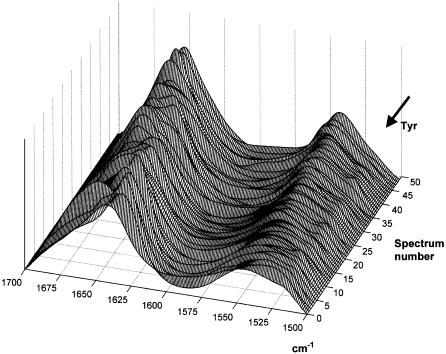
FIGURE 1.
ATR-FTIR spectra of a series of 50 proteins sorted in order of increasing _α_-helix content. A baseline drawn between the spectra data points at 1700 and 1500 cm−1 has been subtracted. The spectra have been rescaled to the same area below the amide I–II region as described in Materials and Methods. The arrow indicates the wavenumber of the tyrosine side-chain contribution (1516 cm−1).
Protein secondary structure evaluation from DSSP output
The secondary structures of the 50 proteins used here were determined with the DSSP program (36) and have been listed elsewhere (33). There are eight assignments made by DSSP. Six are familiar to protein chemists: _α_-helix (denoted by H), 310 helix (G), _π_-helix (I), _β_-sheet (E), turn (T), and unassigned structure (indicated by a blank space in the DSSP program output). Unassigned structure has been referred to by many names, such as irregular, other, disordered, random, or coil. Because of their low frequency, _π_-helices were not considered in this study. The small range of variation found for the 310 helices also prevents statistically meaningful results to be obtained on the present set of proteins even though they are characterized by specific IR features (37).
Spectroscopic data collection and processing
All protein preparations were desalted by dialysis or size-exclusion chromatography. Attenuated total reflection infrared (ATR-FTIR) spectra were obtained on a Bruker IFS55 FTIR spectrophotometer (Bruker, Ettlingen, Germany) equipped with a MCT detector (broadband 120,000–420 cm−1, liquid N2 cooled, 24 h hold time) at a resolution of 2 cm−1 with an aperture of 3.5 mm and acquired in the double-sided, forward-backward mode. The spectrometer was placed on vibration-absorbing sorbothane mounts (Edmund Industrial Optics, Barrington, NJ). Two levels of zero filling of the interferogram before Fourier transform allowed encoding the data every 1 cm−1. The spectrometer was continuously purged with dry air (Model 75-62, Whatman, Haverhill, MA). For better stability, the purging of the spectrometer optic compartment (50 l/min) and of the sample compartment (100 l/min) were dissociated and controlled independently by flowmeters (Fisher Bioblock Scientific, Illkirch, France). The internal reflection element was a 52 × 20 × 2 mm trapezoidal germanium ATR plate (ACM, Villiers St. Frédéric, France) with an aperture angle of 45° yielding 25 internal reflections. The germanium crystals were washed in Superdecontamine (Intersciences, Brussels, Belgium), a lab detergent solution at pH 13, rinsed with distilled water, washed with methanol, then with chloroform and finally placed for 2 min in a plasma cleaner PDC23G (Harrick, Ossining, NY) working under reduced air pressure. Measurements were carried out at room temperature. Thin films were obtained by slowly evaporating a sample solution containing 100 _μ_g of protein on one side of the ATR plate under a stream of nitrogen. The contribution of water vapor from infrared spectra was subtracted using a scaling factor determined from the integrated absorbance of the 1717 or 1772 cm−1 bands.
Analysis methods
All the data processing was performed with a homemade software running under the MatLab 7.1 environment (The MathWorks, Natick, MA).
Linear regression models—cross-validation
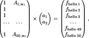
In an attempt to build a model describing the secondary structure content, we used the absorbance values at selected frequencies. The simplest model relates the absorbance at one wavenumber to one secondary structure content. For the sake of simplicity, we consider the helix content in the following description. The model used is linear in the absorbance _A_j,wi where j is the spectrum number and _w_i the wavenumber. Here, A represents the absorbance of the rescaled spectra (see below). The model includes a constant, _a_1, and a proportionality factor (_a_2). At any given wavenumber _w_i, the helix fractional content _f_helix j is tentatively related to the absorbance _A_j,wi by _f_helix j = _a_1 + _a_2 _A_j,wi. For all the spectra, this can be written as
 |
(1) |
|---|
which can be easily solved for the best constants _a_k (with k = 1,2) in the least-square sense.
For identifying the best wavenumber, cross-validation was carried out. For this purpose, each spectrum was removed in turn from the database, a model was built from the remaining spectra, and the helical content corresponding to the spectrum was predicted yielding a predicted concentration _f_helix j. This procedure was repeated for all the spectra in the series. In turn, Eq. 1 containing 49 spectra was solved 50 times, yielding 50 sets of constants _a_1 and _a_2 that were used for predicting the helix content for the protein whose spectrum was removed. The standard deviation of the difference between the predicted values _f_helix j and the real _f_refhelix j values (j = 1–50) was used to evaluate the quality of the model at wavenumber _w_i.
The whole cross-validation procedure was then repeated for every wavenumber _w_i of the spectra from 4000 to 800 cm−1 by steps of 1 cm−1. The wavenumber with the smallest standard deviation was retained for further building of a more accurate model containing a second absorbance value in an ascending stepwise manner. The first selected wavenumber is called _w_1 below.
Ascending stepwise model building
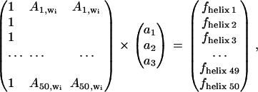
For the ascending stepwise building of the model, the best wavenumber _w_1 selected in the cross-validation process described above was retained in the model and a second one was added as described in Eq. 2 for the _α_-helix content model:
 |
(2) |
|---|
As described before, the cross-validation procedure was used, the constants _a_1–_a_3 were obtained and used to predict the secondary structure _f_helix j from Eq. 2. The standard deviation of the difference between the predicted values _f_helix j and the reference _f_refhelix j values (j = 1–50) was used to evaluate the quality of the new model. The cross-validation procedure was repeated for every wavenumber _w_i of the spectra. The wavenumber with the smallest standard deviation was retained. At this stage, the model contained two frequencies of _w_1 and _w_2.
The entire procedure was repeated up to eight times in this study, defining the eight best frequencies for the description of a secondary structure.
Finally, the analysis was repeated for all the secondary structures considered.
Quadratic models in the absorbance
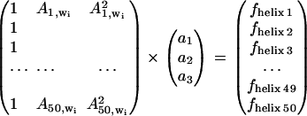
To take into account potential nonlinearities, we also investigated models linear in the absorbance _A_j, wi and the square of the absorbance  , where j is the spectrum number and _w_i the wavenumber. The one-wavenumber model now includes a constant, _a_1, and two proportionality factors (_a_2 and _a_3), one for the absorbance and one for the square of the absorbance. For the _α_-helix content, this one-wavenumber (_w_i) model can be written
 |
(3) |
|---|
It can be easily solved for the best constants _a_k (k = 1–3) in the least-square sense. Cross-validation was performed as described before. The whole cross-validation procedure was then repeated for every wavenumber _w_i of the spectra (every 1 cm−1). The wavenumber with the smallest standard deviation was retained for further building of a more accurate model containing a second absorbance value in an ascending stepwise manner.
For the ascending stepwise building of the model, the best wavenumber _w_1 selected in the cross-validation process described above was retained in the model and a second one was added. The same procedure was repeated up to eight times in this study, defining the eight best frequencies for the description of a secondary structure.
Normalization
Two types of normalizations were performed in this work:
- Area normalization consisted in rescaling the spectra so that the area between the spectra and the baseline drawn between the spectrum point at 1700 and 1500 cm−1 was 10,000.
- Point normalization consisted in dividing the spectrum by the absorbance at one wavenumber.
In this work, the spectra were normalized in turn by the absorbance at each wavenumber (every 1 cm−1) and the whole process of cross-validation described above restarted. The normalization wavenumber yielding the lowest standard deviation was determined for each secondary structure.
Synchronous map
Generalized two-dimensional correlation spectra were calculated according to Noda (38,39). The validity of unexpected cross-peak such as the correlation between 1655 cm−1 and 2950 cm−1 was verified as described by Buchet et al. (40).
RESULTS AND DISCUSSION
The ATR-FTIR spectra of the 50 proteins of the database described in Materials and Methods (see also Appendix) are presented in Fig. 1. Spectra have been scaled to an identical area under amides I and II (1700–1500 cm−1) and a linear baseline subtracted between these two frequencies. Even though the spectra are sorted for increasing _α_-helix content, the maximum of amide I appears to be shifted toward ∼1655 cm−1 as the _α_-helix content increases in a quite complex manner. This figure illustrates the complexity of the band shape-structure relationship. Protein #5 is notably out of the general pattern as it is neither helical nor sheet but fully disordered. The shoulder of variable intensity at 1516 cm−1 can be safely assigned to tyrosine. The side-chain contribution to the IR spectrum is a key issue and will be discussed later in this article.
Correlations
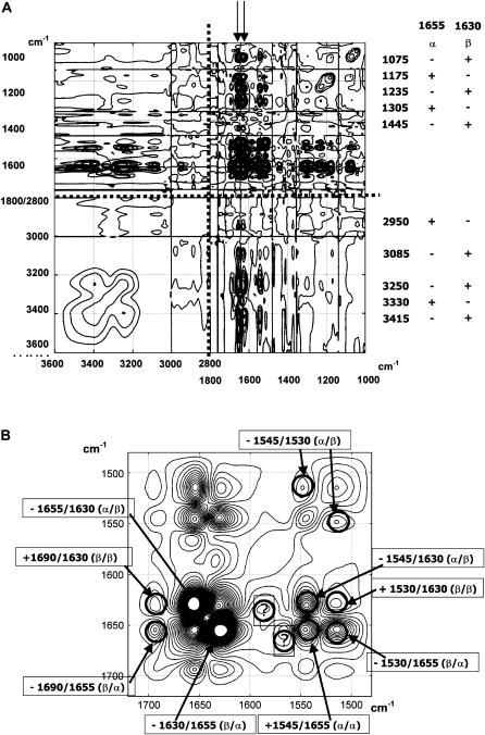
How much independent information is present in the spectra is an important question. Fig. 2 A reports the correlations existing in the 3600–2800 + 1800–1000 cm−1 regions of the spectrum. Spectra have been normalized on the 1700–1600 cm−1 amide I–II region as described in Materials and Methods. The two arrows in Fig. 2 A are located at 1655 cm−1 (assigned to _α_-helix) and 1630 cm−1 (assigned to _β_-sheet). The 1655 cm−1 band is positively correlated with bands at 1175, 1305, 2950, and 3330 cm−1 while the 1630 cm−1 band is positively correlated with bands at 1075, 1235, 1445, 3085, 3250, and 3415 cm−1. Bands below 1400 cm−1 could be roughly assigned to amide III and bands above 3000 cm−1 to amides A and B. The distinct correlation found at 2950 cm−1 in the C–H stretching region remains unexplained. The details of the correlations existing in the amide I–II region appear in Fig. 2 B. Fig. 2 B indicates that numerous correlations exist in the amide I–II region, indicating the presence of redundant information. The most obvious correlations are labeled on the figure and are in line with previous assignments for the different secondary structure contributions in the amide I–II range of the infrared spectrum (e.g., (5)). Two bands, 1655 and 1545, can be assigned to the _α_-helix structure, and the 1630 and 1530 cm−1 bands can be assigned to the _β_-sheet structure. Off-diagonal contributions distinctly show the high wavenumber contribution of the _β_-sheet at 1690 cm−1. The negative sign of the correlation also explicitly indicates that the _α_-helix and _β_-sheet are mutually exclusive. This can be easily rationalized, as the sum of both was found to be roughly constant in the database (33). Two correlations bands (1570/1640 and 1585/1635 cm−1) remain unassigned. The well-known relation between amino acid composition and secondary structure could imprint its mark on the correlation plot in infrared spectroscopy. Overall, the large number of correlations revealed in this study indicates a large degree of redundancy in the different regions of the spectra.
FIGURE 2.
Synchronous correlation (A) for the 3600–2800 and 1800–1000 cm−1 regions (separated by dotted lines). The right column indicates the frequencies of the bands correlated with the 1655 and 1630 amide I components (arrows) and the sign of the correlation. (B) Enlarged over the amide I–II region (1720–1480 cm−1). To better visualize weaker correlations in panel A, level curves have been drawn more densely near zero.
Secondary structure prediction
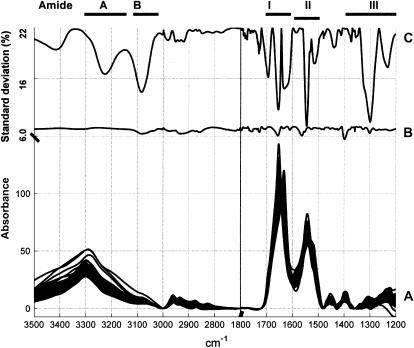
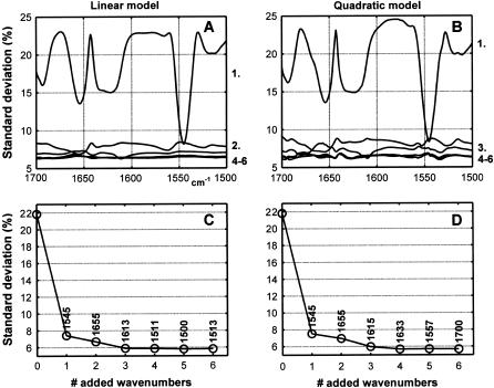
Fig. 3 A reports the series of 50 spectra present in the database. Fig. 3 C reports the standard deviation for the prediction (called here the standard error of prediction) of the _α_-helix content for a model including the absorbance at a single wavenumber as a function of the selected wavenumber. This result has been obtained after cross-validation, as explained in Materials and Methods. This figure reveals the capability of the absorbance at every wavenumber (every 1 cm−1 here) to predict the _α_-helix content according to a simple model described in Eq. 1. It also reveals that, beside the amide I region of the spectra usually used for this purpose, the absorbance in the amide A, B, and more definitively amide III regions are strongly correlated with the _α_-helix content, as was recently reported in Surewicz and Mantsch (41). In line with the results reported in Fig. 2, Fig. 3 C indicates that the best wavenumber to use to predict the _α_-helix content is 1545 cm−1—which is, surprisingly, in the amide II range. It is positively correlated with the well-known 1655 cm−1 helix band (Fig. 2 B), but better correlated than the latter with the _α_-helix content. It has long been recognized that the amide II band is conformationally sensitive. However, the dependence of the amide II band shape on secondary structure is complex, so it has not been considered systematically for quantitative analyses. This finding is also in agreement with the recent article by Oberg et al. (42), suggesting for the first time that the amide II band could be used alone for protein _α_-helix content determination. When using this single wavenumber, the standard deviation drops from 22%; i.e., the standard deviation of the helix content in the whole database drops to 7.4%. When this wavenumber is permanently kept in the model while another one is added according to Eq. 2, a more elaborated and accurate model is built. The resulting standard error of prediction appears in Fig. 3 B. This curve reveals that, once the 1545 cm−1 wavenumber is incorporated in the model, the addition of a second wavenumber brings much less improvement. Importantly, most of the information initially present in the amide A, B, and amide III region is now largely irrelevant, because it is redundant with the 1545 cm−1 information. This could be expected from the correlation map drawn in Fig. 2. The only exception is the band near 1400 cm−1 whose contribution is now the largest, but roughly similar to the additional information still contained in the amide II at 1563 cm−1 and in the amide I at 1655 cm−1. Because the 1400 cm−1 band information is itself largely redundant with the 1655 cm−1 information, we shall consider only the amide I and II regions in the rest of this article since the other ones are typically difficult to use in the presence of other molecules (buffer, lipids, etc.). The stepwise procedure presented here allows the monitoring of the quality of the model as more wavenumbers are added in the model. Fig. 4, A and C, demonstrates in the case of the _α_-helix that in the cross-validation mode, the first wavenumber contains most of the information useful for the prediction of the _α_-helix content. The standard error of prediction is 6.6 and 5.9%, respectively, for a two-wavenumber and a three-wavenumber linear model. Importantly, Fig. 4 clearly indicates that, at most, three wavenumbers contain all the nonredundant information since addition of more wavenumbers does not improve the prediction any further. Interestingly, Fig. 4, B and D, also indicates that addition of quadratic terms (Eq. 3) does not significantly improve the prediction (at most by 0.1%). This is also the case for the other structures (not shown). This result demonstrates that no large nonlinearity is present in the ATR spectra. A different result was obtained for circular dichroism spectroscopy (43).
FIGURE 3.
Information content in the ATR-FTIR spectra pertaining to the _α_-helix content in the proteins. (A) Series of the spectra in the database presented between 3500 and 2700 + 1800 – 1200 cm−1. (B) Evolution of the standard error of prediction for the _α_-helix content for a two-wavenumber model. (C) Evolution of the standard error of prediction for the _α_-helix content for a one-wavenumber model. The smaller values indicate where the model is the most accurate. The best wavenumber determined on the line C is kept in the model and a second is added. The indications on top of the figure localize the bands called amide A, amide B, amide I, amide II, and amide III.
FIGURE 4.
(A) Evolution of the standard error of prediction for the _α_-helix content for a linear model containing one wavenumber (the model is %helix = _a_0 + _a_1 × _A_1545 cm−1, where _a_0 and _a_1 are determined according to Eq. 1), top curve, two wavenumbers (the model is %helix = _a_0 + _a_1 × _A_1545 cm−1 + _a_2 × _A_1656 cm−1, where _a_0, _a_1, and _a_2 are determined according to Eq. 2) and 3–6 wavenumbers. The smallest values indicate where the model is the most accurate. (B) As for A, but the quadratic model described by Eq. 3 is applied. (C) Evolution of the best standard error of prediction for the _α_-helix content for a linear model containing 1–6 wavenumbers (see A). Panel D is essentially the same as panel C, but it was built for the quadratic model (see B). A linear baseline has been drawn between the spectrum data points at 1700 and 1600 cm−1 and subtracted. The area of every spectrum was rescaled to an arbitrary value of 10,000.
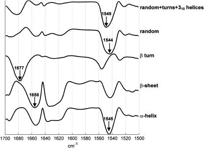
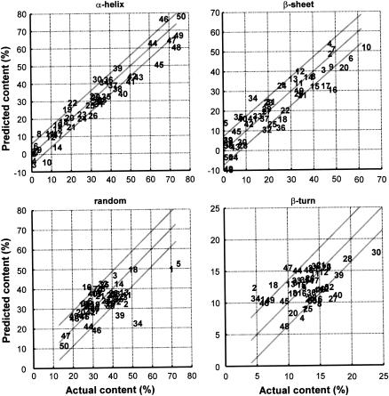
Although there are no more than three wavenumbers that contain useful independent information for one secondary structure, Fig. 5 shows that a different set of three wavenumbers is absolutely required for each individual secondary structure. The best wavenumber for prediction is found at 1545 cm−1 for the _α_-helix, 1656 cm−1 for the _β_-sheet, 1677 cm−1 for the _β_-turn, and 1544 cm−1 for the random structure. Amazingly, the _β_-sheet sheet content is best described by the absorbance at 1656 cm−1, a wavenumber assigned to _α_-helix structures. In fact, this band is negatively correlated with the _β_-sheet contribution at 1630 cm−1 (Fig. 2 B). In turn, the similarity between the _α_-helix and _β_-sheet profiles (Fig. 5) might be understood in view of the strong (negative) correlation existing between the content of the two structures (Fig. 2). In other words, determining one of them brings a good prediction for the other. This is graphically illustrated in the Supplementary Material. As discussed earlier, this property is also a general property of the structure distribution in the PDB (33). At the opposite, the prediction error profiles of the _β_-turn and random structures reported in Fig. 5 have very distinct and unique features. The standard errors of prediction are reported in Table 1 for three-wavenumber linear and quadratic models. It can be observed that the quadratic models are doing only slightly better. Considering the fact that for models including three wavenumbers, the quadratic ones contain seven constants instead of three for the linear models, this improvement was considered here as not significant. The results for the 50 proteins are reported in Fig. 6 for the three frequency linear models. The corresponding equations are reported in Table 1 (see also Table 2). It can be observed that the systematic overevaluation of the _β_-sheet content for mainly helical proteins described earlier (see Introduction) does not occur here.
FIGURE 5.
Plot of the standard deviation evolution as a function of the wavenumber included in a one-wavenumber linear model (Eq. 1). For the clarity of the figure, the curves have been rescaled and offset. The arrows point to the best frequencies identified for each spectrum.
TABLE 1.
Standard errors of prediction for area-normalized spectra
| RMS | Cross-valid lin1 | Cross-valid lin2 | Cross-valid quad3 | Direct valid | Frequencies in model | Model →% of the secondary structure | |
|---|---|---|---|---|---|---|---|
| _α_-Helix | 21.8 | 5.9 | 5.5 | 5.9 | 5.4 | 1545–1655–1613 | −179.45 + 2.030 × A1545 + 0.431 × A1655 + 0.828 × A1613 |
| _β_-Sheet | 17.6 | 7.3 | 7.0 | 6.5 | 6.6 | 1656–1634–1691 | 26.31 − 0.451 × A1656 + 0.335 × A1634 + 0.586 × A1691 |
| _β_-Turns | 4.2 | 3.6 | 3.7 | 3.0 | 3.2 | 1677–1528–1577 | −30.49 + 0.428 × A1676 + 0.322 × A1528 + 0.141 × A1577 |
| Random | 11.4 | 8.8 | 9.3 | 8.9 | 7.9 | 1544–1627–1691 | 178.56 − 1.578 × A1544 − 0.332 × A1627 − 0.735 × A1691 |
| 310-Helix | 3.2 | 3.1 | 3.1 | 3.0 | 2.9 | 1631–1694–1625 | 5.077 − 0.198 × A1631 + 0.440 × A1694 + 0.160 × A1625 |
| Random + turns + 310-helices | 12.8 | 8.2 | 8.6 | 8.1 | 7.3 | 1549–1629–1513 | 224.544 − 2.010 × A1549 − 0.345 × A1629 − 0.775 × A1513 |
FIGURE 6.
Predicted versus actual secondary structure content. Predictions were obtained in cross-validation, using the best three wavenumbers determined and according to the simple expression reported in Table 1. The numbers refer to the protein number code (see Appendix). The lines represent a linear fit and the limits set by ±1 SD.
Unlike some experiments such as IR laser experiments, in which only a few wavenumbers can be monitored (e.g., (44)), the present work brings a potentially very useful method to evaluate secondary structures. It should be emphasized that as far as a single wavenumber is concerned, all the secondary structure information content appears on Fig. 5. If the user wants to force the model to start with a preset wavenumber, the present approach can be used to determine the next-best wavenumbers to monitor. For instance, when the _α_-helix is tested at 1630 cm−1, the prediction is not good (standard error of prediction = 15%). Letting the ascending stepwise method search for the next best wavenumber largely restores the quality of the prediction. In this particular case, forcing the model to start with 1630 cm−1 results in the selection of 1656 and 1611 cm−1 as the second and third wavenumber introduced, with a standard error of prediction of 6.3% for the _α_-helix structure in cross-validation mode—not dramatically far from the best result reported in Table 1 (5.5%). Another related question is how best we can predict all secondary structures using only one set of wavenumbers. If the criterion is to minimize the average standard error of prediction over the different secondary structures, it is possible to develop a model using the same wavenumbers for all the structures (Table 3). It can be observed that even though the results are not exactly as good as these generated by the best individual models, the predictions are fairly good and could be used for structural studies. In the course of this investigation, we showed that adding more than three wavenumbers to the model does not improve its quality for any of the secondary structures considered (data not shown).
TABLE 3.
Single model standard errors of prediction for area-normalized spectra
| RMS | Cross-valid lin | Direct valid | Frequencies in model | Model →% of the secondary structure | |
|---|---|---|---|---|---|
| _α_-Helix | 21.8 | 6.3 | 5.8 | – | −218.813 + 2.473 × A1545 + 0.565 × A1655 + 1.121 × A1611 |
| _β_-Sheet | 17.6 | 7.6 | 7.0 | 1545–1655–1611 | 134.940 + 0.3861 × A1545 − 0.859 × A1655 − 0.741 × A1611 |
| _β_-Turns | 4.2 | 3.6 | 3.2 | – | −14.043 + 0.475 × A1545 + 0.380 × A1655 − 0.650 × A1611 |
| Random | 11.4 | 8.9 | 7.9 | – | 216.0146 − 1.285 × A1545 − 0.457 × (A1655) − 1.019 × A1611 |
Database subset selection
It has been reported previously that better evaluations of secondary structure contents may be obtained if the training set is restricted to spectra presenting a high similarity with the tested spectrum. To test this possibility, we repeated the whole analysis described so far but restricting the training set to the 25 closest spectra as measured by the Euclidian distance. The results are reported in Table 1. Some improvement was obtained for the _α_-helix and _β_-sheet structures. At the opposite, the prediction was degraded for the other structures. Selecting smaller or larger subsets for the training did not bring any further improvement (not shown).
Derivatives and baselines
The preprocessings to be applied to the spectra remains a question for the spectroscopist. The ascending stepwise procedure was applied to first derivatives of the spectra. The results in terms of prediction accuracy are exactly the same as these presented here. Furthermore, when a baseline joining points of the spectra every 10 cm−1 was drawn and subtracted, again the accuracy of the secondary structure prediction was found to be the same (within 0.1%). These two results (not shown) indicate that there is no room for further baseline-related improvement.
Point normalization
In place of the area normalization of the spectra, it might be tempting to rescale the spectra so that the absorbance at a given wavelength is equal, as recently suggested for CD spectra (43). Such a procedure is even simpler than the previous one (area normalization) and potentially eliminates scaling artifacts due to spurious absorbances, in particular because of side-chain contributions in the amide I–II region or other artifacts. To test this possibility we reproduced the entire cross-validation procedure for spectra rescaled every 1 cm−1. All wavenumbers (every cm−1) were used for normalization in turn and the whole process described above restarted. Results are reported in Table 1. For the _α_-helix, the best normalization wavenumber was found at 1641 cm−1 but the standard error of prediction was 6.9% instead of 5.9% for area normalization. For the _β_-sheet, the best normalization wavenumber was found at 1653 cm−1 and the standard deviation for the prediction fell at 6.4%; i.e., a significant improvement over the area normalization reported in Table 1 (7.3%). This result suggests that different spectral preprocessing must be applied to obtain the best predictions.
Size of the protein database
The accuracy obtained in cross-validation (Table 1) is not as good as for some early works (e.g., (1)). The reason for this is that the protein database used here has been built to avoid redundant structures and to be as representative as possible of the diversity of the folds that have been described in crystallized proteins (33). In turn, unique structures are more frequent. We could easily decrease the standard error of prediction from 5.9% for the _α_-helix content to 4.2% by selecting a subset of 40 proteins, but the standard error of prediction for the removed protein then increases to 9.7% (not shown). Such an improvement is therefore not desirable, and this result emphasizes the importance of the selection of the protein present in the database. Including unique structures obviously increases the cross-validation standard error of prediction but also increases the capability of the database to describe an unknown protein, in agreement with previous observations on the generalization problem (20).
Side chains
The contribution of the side chains to the spectrum of each protein in the amide I–II region of the IR spectrum was computed and scaled as described previously (45,46). To achieve this result, our software read the PDB files corresponding to each protein and extracted the secondary structure and the amino acid composition. The individual contributions of every side chain was rebuilt according to the data available in the literature (47–50) reviewed in Goormaghtigh et al. (51) and Barth and Zscherp (52). To illustrate the variability of the side-chain contributions, the side-chain contributions for the 50 proteins were overlaid (see Supplementary Material). Even though these contributions usually represent <10% of the amide area, the overlay of the spectra indicates that the individual contributions can be significantly different in shape, due to differences in amino acid composition. Such corrections have been found to be necessary for the correct evaluation of the amide II band area in 1H/2H exchange kinetic experiments (53–61). It must be stressed that the side-chain contributions reported correspond to protein in solution. Yet, we could observe in several 1H/2H exchange kinetic experiments (53–61) that the reported contributions match the experimental spectra features revealed either by Fourier self-deconvolution or by the exchange process. In the present case, our investigation shows that subtraction of the side-chain contributions slightly degrades the prediction for all secondary structure types (not shown). This result can be rationalized if we think about the various sources of errors that cannot be avoided in the process of side-chain contribution building and subtraction. Such errors appear to be too large in front of the sensitivity required for secondary structure determination, but small when only the area of the amide II band must be evaluated in 1H/2H exchange kinetic experiments.
Protein film versus protein solution
It is generally accepted that infrared spectra of proteins in films and in solution may display distinct differences, even though both systems are widely used. These differences appear to be due to the presence or absence of the water of buffer molecules that imprint their mark on the spectra. Yet, a number of experimental evidences indicate that studying the structure of proteins and lipids on thin film by ATR is a valid approach: These evidences include measurements on both systems of enzyme activity, effect of pH and protein conformation based on amide band shapes, and hydrogen/deuterium kinetics. These evidences have been extensively reviewed in Goormaghtigh et al. (27). For this work we have attempted to validate the approach described here on the same set of proteins in aqueous solution. We found that the structural information content is the same in films and in solution, i.e., the prediction we obtain with three wavenumbers is of the same quality (same error of prediction within <1%) for both systems even though the spectral shape is slightly different. In turn, a model specific for the second situation must be built for optimal prediction.
CONCLUSIONS
The stepwise approach described here has the advantage of helping the understanding of the correlation between the various IR frequencies and the secondary structures, as the relevant wavenumber regions are clearly visible. This work also clearly demonstrates that, among the 3201 frequencies tested here (from 4000 to 800 by steps of 1 cm−1), only three frequencies contain all the information that is available to predict the secondary structure of the proteins. Once these three frequencies are included in a simple linear model, none of the other data points of the IR spectrum contains any additional useful information for the prediction of the secondary structures. This approach avoids forcing less-well correlated frequencies to be introduced in the model. It could be argued that the partial least-squares approach should be more robust than the one currently used. Yet, the high quality of the spectra available now makes it possible to use only a few single points of the spectrum for the analysis.
Interestingly, the optimal preprocessings are found to be different for the different secondary structures. Similarly, the optimal frequencies used are specific for every secondary type. This indicates that although no more than three wavenumbers are significant for one secondary structure, the information is distinct for the different secondary structure types, notwithstanding the large degree of correlation that may exist between some of them.
SUPPLEMENTARY MATERIAL
An online supplement to this article can be found by visiting BJ Online at http://www.biophysj.org.
Supplementary Material
[Supplemental]
TABLE 2.
Standard errors of prediction for point-normalized spectra
| RMS | Cross-valid lin1 | Cross-valid lin2 | Cross-valid quad3 | Direct valid | Norm frequency | Frequencies in model | Model →% of the secondary structure | |
|---|---|---|---|---|---|---|---|---|
| _α_-Helix | 21.8 | 6.9 | 6.6 | 7.2 | 6.2 | 1641 | 1545–1565–1530 | −37.082 + 223.655 × A1545 − 86.095 × A1565 − 82.481 × A1530 |
| _β_-Sheet | 17.6 | 6.6 | 6.6 | 6.6 | 6.1 | 1653 | 1638–1530–1656 | −68.570 + 70.386 × A1638 − 21.433 × A1530 + 32.581 × A1656 |
| _β_-Turns | 4.2 | 3.4 | 3.7 | 3.6 | 3.1 | 1565 | 1685–1563–1687 | 102.655 + 31.310 × A1685 − 94.161 × A1563 − 23.584 × A1687 |
| Random | 11.4 | 8.6 | 10.4 | 10.4 | 8.4 | 1552 | 1679–1553–1687 | −569.019 + 87.979 × A1679 + 593.514 × A1553 − 89.106 × A1687 |
| 310-Helix | 3.2 | 2.8 | 3.0 | 2.8 | 2.6 | 1545 | 1546–1547– 1512 | 1147.907 − 2192.463 × A1546 + 1058.537 × A1547 − 15.803 × A1512 |
| Random + turns + 310-helices | 12.8 | 8.0 | 9.1 | 10.3 | 7.2 | 1543 | 1671–1587–1541 | −252.957 + 47.236 × A1671 + 47.690 × A1587 + 242.377 × A1541 |
Acknowledgments
Dr. Goormaghtigh is Research Director and V. Raussens Research Associate of the Belgian National Fund For Scientific Research.
This work was funded by a grant from Action de Recherches Concertées, Belgium.
APPENDIX
1
Trypsin inhibitor (soy bean)
2
Avidin
3
Erabutoxin b
4
Concavalin A
5
Metallothionein II
6
_α_-hemolysin (_α_-toxin)
7
Lectin (lentil)
8
Superoxide dismutase (Cu, Zn)
9
Immunoglobulin-γ
10
Xylanase
11
Trypsinogen
12
_α_-Chymotrypsinogen A
13
Carbonic anhydrase
14
Thaumatin
15
Pepsinogen
16
Rennin (chymosin b)
17
Pepsin
18
Trypsin inhibitor (BPTI)
19
Ubiquitin
20
Monellin
21
Ribonuclease A
22
Ricin
23
Papain
24
Alcohol dehydrogenase
25
Glucose oxidase
26
Ovalbumin
27
Subtilisin BPN′ (nagarse)
28
_α_-Lactalbumin
29
Subtilisin Carlsberg
30
Lysozyme
31
Penicillin amidohydrolase
32
DD-transpeptidase
33
Lipoxygenase-1
34
Phosphoglyceric kinase
35
Peroxidase
36
Dihydropteridine reductase
37
Triose phosphate isomerase
38
Insulin
39
Cytochrome C
40
Phospholipase A2
41
Superoxide dismutase (Fe)
42
Glutathione S-transferase
43
Parvalbumin
44
Citrate synthetase
45
Troponin
46
Apolipoprotein E3, N-terminal domain (residues 1–183)
47
Hemoglobin
48
Ferritin (apo)
49
Colicin A, C-terminal domain
50
Myoglobin
The proteins are identified by their number in the figures of this article.
References
- 1.Byler, D. M., and H. Susi. 1986. Examination of the secondary structure of proteins by deconvolved FTIR spectra. Biopolymers. 25:469–487. [DOI] [PubMed] [Google Scholar]
- 2.Cabiaux, V., R. Brasseur, R. Wattiez, P. Falmagne, J. M. Ruysschaert, and E. Goormaghtigh. 1989. Secondary structure of diphtheria toxin and its fragments interacting with acidic liposomes studied by polarized infrared spectroscopy. J. Biol. Chem. 264:4928–4938. [PubMed] [Google Scholar]
- 3.Prestrelski, S. J., K. A. Pikal, and T. Arakawa. 1995. Optimization of lyophilization conditions for recombinant human interleukin-2 by dried-state conformational analysis using Fourier-transform infrared spectroscopy. Pharm. Res. 12:1250–1259.8570516 [Google Scholar]
- 4.Goormaghtigh, E., V. Cabiaux, and J. M. Ruysschaert. 1990. Secondary structure and dosage of soluble and membrane proteins by attenuated total reflection Fourier-transform infrared spectroscopy on hydrated films. Eur. J. Biochem. 193:409–420. [DOI] [PubMed] [Google Scholar]
- 5.Goormaghtigh, E., V. Cabiaux, and J. M. Ruysschaert. 1994. Determination of soluble and membrane protein structure by Fourier transform infrared spectroscopy. III. Secondary structures. Subcell. Biochem. 23:405–450. [DOI] [PubMed] [Google Scholar]
- 6.Jackson, M., and H. H. Mantsch. 1995. The use and misuse of FTIR spectroscopy in the determination of protein structure. Crit. Rev. Biochem. Mol. Biol. 30:95–120. [DOI] [PubMed] [Google Scholar]
- 7.Surewicz, W. K., and H. H. Mantsch. 1988. New insight into protein secondary structure from resolution- enhanced infrared spectra. Biochim. Biophys. Acta. 952:115–130. [DOI] [PubMed] [Google Scholar]
- 8.Haris, P. I., D. Chapman, and G. Benga. 1995. A Fourier-transform infrared spectroscopic investigation of the hydrogen-deuterium exchange and secondary structure of the 28-kDa channel-forming integral membrane protein (CHIP28). Eur. J. Biochem. 233:659–664. [DOI] [PubMed] [Google Scholar]
- 9.Jap, B. K., M. F. Maestre, S. B. Hayward, and R. M. Glaeser. 1983. Peptide-chain secondary structure of bacteriorhodopsin. Biophys. J. 43:81–89. [DOI] [PMC free article] [PubMed] [Google Scholar]
- 10.Van Hoek, A. N., M. Wiener, S. Bicknese, L. Miercke, J. Biwersi, and A. S. Verkman. 1993. Secondary structure analysis of purified functional CHIP28 water channels by CD and FTIR spectroscopy. Biochemistry. 32:11847–11856. [DOI] [PubMed] [Google Scholar]
- 11.Baumruk, V., P. Pancoska, and T. A. Keiderling. 1996. Predictions of secondary structure using statistical analyses of electronic and vibrational circular dichroism and Fourier transform infrared spectra of proteins in H2O. J. Mol. Biol. 259:774–791. [DOI] [PubMed] [Google Scholar]
- 12.Lee, D. C., P. I. Haris, D. Chapman, and R. C. Mitchell. 1990. Determination of protein secondary structure using factor analysis of infrared spectra. Biochemistry. 29:9185–9193. [DOI] [PubMed] [Google Scholar]
- 13.Pribic, R., I. H. van Stokkum, D. Chapman, P. I. Haris, and M. Bloemendal. 1993. Protein secondary structure from Fourier transform infrared and/or circular dichroism spectra. Anal. Biochem. 214:366–378. [DOI] [PubMed] [Google Scholar]
- 14.Sarver, R. W., Jr., and W. C. Krueger. 1991. An infrared and circular dichroism combined approach to the analysis of protein secondary structure. Anal. Biochem. 199:61–67. [DOI] [PubMed] [Google Scholar]
- 15.Dousseau, F., and M. Pezolet. 1990. Determination of the secondary structure content of proteins in aqueous solutions from their amide I and amide II infrared bands. Comparison between classical and partial least-squares methods. Biochemistry. 29:8771–8779. [DOI] [PubMed] [Google Scholar]
- 16.Rahmelow, K., and W. Hubner. 1996. Secondary structure determination of proteins in aqueous solution by infrared spectroscopy: a comparison of multivariate data analysis methods. Anal. Biochem. 241:5–13. [DOI] [PubMed] [Google Scholar]
- 17.Vedantham, G., H. G. Sparks, S. U. Sane, S. Tzannis, and T. M. Przybycien. 2000. A holistic approach for protein secondary structure estimation from infrared spectra in H2O solutions. Anal. Biochem. 285:33–49. [DOI] [PubMed] [Google Scholar]
- 18.Hering, J. A., P. R. Innocent, and P. I. Haris. 2002. Automatic amide I frequency selection for rapid quantification of protein secondary structure from Fourier transform infrared spectra of proteins. Proteomics. 2:839–849. [DOI] [PubMed] [Google Scholar]
- 19.Hering, J. A., P. R. Innocent, and P. I. Haris. 2002. An alternative method for rapid quantification of protein secondary structure from FTIR spectra using neural networks. Spectrosc. Int. J. 16:53–69. [Google Scholar]
- 20.Severcan, M., P. I. Haris, and F. Severcan. 2004. Using artificially generated spectral data to improve protein secondary structure prediction from Fourier transform infrared spectra of proteins. Anal. Biochem. 332:238–244. [DOI] [PubMed] [Google Scholar]
- 21.Hering, J. A., P. R. Innocent, and P. I. Haris. 2004. Towards developing a protein infrared spectra databank (PISD) for proteomics research. Proteomics. 4:2310–2319. [DOI] [PubMed] [Google Scholar]
- 22.Baello, B. I., P. Pancoska, and T. A. Keiderling. 2000. Enhanced prediction accuracy of protein secondary structure using hydrogen exchange Fourier transform infrared spectroscopy. Anal. Biochem. 280:46–57. [DOI] [PubMed] [Google Scholar]
- 23.Venyaminov, S. Y., J. F. Hedstrom, and F. G. Prendergast. 2001. Analysis of the segmental stability of helical peptides by isotope-edited infrared spectroscopy. Proteins. 45:81–89. [DOI] [PubMed] [Google Scholar]
- 24.Arrondo, J. L., J. Castresana, J. M. Valpuesta, and F. M. Goni. 1994. Structure and thermal denaturation of crystalline and noncrystalline cytochrome oxidase as studied by infrared spectroscopy. Biochemistry. 33:11650–11655. [DOI] [PubMed] [Google Scholar]
- 25.Arrondo, J. L. R., I. Etxabe, U. Dornberger, and F. M. Goni. 1994. Probing protein conformation by infrared spectroscopy. Biochem. Soc. Trans. 22:S380. [DOI] [PubMed] [Google Scholar]
- 26.Arrondo, J. L. R., and F. M. Goni. 1999. Structure and dynamics of membrane proteins as studied by infrared spectroscopy. Prog. Biophys. Mol. Biol. 72:367–405. [DOI] [PubMed] [Google Scholar]
- 27.Goormaghtigh, E., V. Raussens, and J. M. Ruysschaert. 1999. Attenuated total reflection infrared spectroscopy of proteins and lipids in biological membranes. Biochim. Biophys. Acta. 1422:105–185. [DOI] [PubMed] [Google Scholar]
- 28.Smith, B. M., and S. Franzen. 2002. Single-pass attenuated total reflection Fourier transform infrared spectroscopy for the analysis of proteins in H2O solution. Anal. Chem. 74:4076–4080. [DOI] [PubMed] [Google Scholar]
- 29.Smith, B. M., L. Oswald, and S. Franzen. 2002. Single-pass attenuated total reflection Fourier transform infrared spectroscopy for the prediction of protein secondary structure. Anal. Chem. 74:3386–3391. [DOI] [PubMed] [Google Scholar]
- 30.Navea, S., R. Tauler, and A. de Juan. 2005. Application of the local regression method interval partial least-squares to the elucidation of protein secondary structure. Anal. Biochem. 336:231–242. [DOI] [PubMed] [Google Scholar]
- 31.Brauner, J. W., C. R. Flach, and R. Mendelsohn. 2005. Quantitative reconstruction of the amide I contour in the IR spectra of globular proteins: from structure to spectrum. J. Am. Chem. Soc. 127:100–109. [DOI] [PubMed] [Google Scholar]
- 32.Orengo, C. A., A. D. Michie, S. Jones, D. T. Jones, M. B. Swindells, and J. M. Thornton. 1997. CATH—a hierarchic classification of protein domain structures. Structure. 5:1093–1108. [DOI] [PubMed] [Google Scholar]
- 33.Oberg, K. A., J. M. Ruysschaert, and E. Goormaghtigh. 2003. Rationally selected basis proteins: a new approach to selecting proteins for spectroscopic secondary structure analysis. Protein Sci. 12:2015–2031. [DOI] [PMC free article] [PubMed] [Google Scholar]
- 34.Harrison, A., F. Pearl, I. Sillitoe, T. Slidel, R. Mott, J. Thornton, and C. Orengo. 2003. Recognizing the fold of a protein structure. Bioinformatics. 19:1748–1759. [DOI] [PubMed] [Google Scholar]
- 35.Orengo, C. A., A. M. Martin, G. Hutchinson, S. Jones, D. T. Jones, A. D. Michie, M. B. Swindells, and J. M. Thornton. 1998. Classifying a protein in the CATH database of domain structures. Acta Crystallogr. D Biol. Crystallogr. 54:1155–1167. [DOI] [PubMed] [Google Scholar]
- 36.Kabsch, W., and S. Sander. 1983. Dictionary of protein secondary structure: pattern recognition of hydrogen-bonded and geometrical features. Biopolymers. 22:2577–2637. [DOI] [PubMed] [Google Scholar]
- 37.Kubelka, J., R. A. Silva, and T. A. Keiderling. 2002. Discrimination between peptide 310- and _α_-helices. Theoretical analysis of the impact of _α_-methyl substitution on experimental spectra. J. Am. Chem. Soc. 124:5325–5332. [DOI] [PubMed] [Google Scholar]
- 38.Noda, I. 1993. Generalized two-dimensional correlation method applicable to infrared, Raman, and other types of spectroscopy. Appl. Spectrosc. 47:1329–1336. [Google Scholar]
- 39.Sasic, S., A. Muszynski, and Y. Ozaki. 2001. New insight into the mathematical background of generalized two-dimensional correlation spectroscopy and the influence of mean normalization pretreatment on two-dimensional correlation spectra. Appl. Spectrosc. 55:343–349. [Google Scholar]
- 40.Buchet, R., Y. Wu, G. Lachenal, C. Raimbault, and Y. Ozaki. 2001. Selecting two-dimensional cross-correlation functions to enhance interpretation of near-infrared spectra of proteins. Appl. Spectrosc. 55:155–162. [Google Scholar]
- 41.Cai, S. W., and B. R. Singh. 2004. A distinct utility of the amide III infrared band for secondary structure estimation of aqueous protein solutions using partial least-squares methods. Biochemistry. 43:2541–2549. [DOI] [PubMed] [Google Scholar]
- 42.Oberg, K. A., J. M. Ruysschaert, and E. Goormaghtigh. 2004. The optimization of protein secondary structure determination with infrared and CD spectra. Eur. J. Biochem. 271:2937–2948. [DOI] [PubMed] [Google Scholar]
- 43.Raussens, V., J. M. Ruysschaert, and E. Goormaghtigh. 2003. Protein concentration is not an absolute prerequisite for the determination of secondary structure from circular dichroism spectra: a new scaling method. Anal. Biochem. 319:114–121. [DOI] [PubMed] [Google Scholar]
- 44.Leeson, D. T., F. Gai, H. M. Rodriguez, L. M. Gregoret, and R. B. Dyer. 2000. Protein folding and unfolding on a complex energy landscape. Proc. Natl. Acad. Sci. USA. 97:2527–2532. [DOI] [PMC free article] [PubMed] [Google Scholar]
- 45.Vigano, C., M. Smeyers, V. Raussens, F. Scheirlinckx, J. M. Ruysschaert, and E. Goormaghtigh. 2004. Hydrogen-deuterium exchange in membrane proteins monitored by IR spectroscopy: a new tool to resolve protein structure and dynamics. Biopolymers. 74:19–26. [DOI] [PubMed] [Google Scholar]
- 46.Goormaghtigh, E., H. H. de-Jongh, and J. M. Ruysschaert. 1996. Relevance of protein thin films prepared for attenuated total reflection Fourier transform infrared spectroscopy: significance of the pH. Appl. Spectrosc. 50:1519–1527. [Google Scholar]
- 47.Chirgadze, Y. N., O. V. Fedorov, and N. P. Trushina. 1975. Estimation of amino acid residue side-chain absorption in the infrared spectra of protein solutions in heavy water. Biopolymers. 14:679–694. [DOI] [PubMed] [Google Scholar]
- 48.Barth, A. 2000. The infrared absorption of amino acid side chains. Prog. Biophys. Mol. Biol. 74:141–173. [DOI] [PubMed] [Google Scholar]
- 49.Venyaminov, S. Y., and N. N. Kalnin. 1991. Quantitative IR spectrophotometry of peptides compounds in water (H2O) solutions. I. Spectral parameters of amino acid residue absorption band. Biopolymers. 30:1243–1257. [DOI] [PubMed] [Google Scholar]
- 50.Rahmelow, K., W. Hubner, and T. Ackermann. 1998. Infrared absorbances of protein side chains. Anal. Biochem. 257:1–11. [DOI] [PubMed] [Google Scholar]
- 51.Goormaghtigh, E., V. Cabiaux, and J. M. Ruysschaert. 1994. Determination of soluble and membrane protein structure by Fourier transform infrared spectroscopy. I. Assignments and model compounds. Subcell. Biochem. 23:329–362. [DOI] [PubMed] [Google Scholar]
- 52.Barth, A., and C. Zscherp. 2002. What vibrations tell us about proteins. Quart. Rev. Biophys. 35:369–430. [DOI] [PubMed] [Google Scholar]
- 53.Raussens, V., J. M. Ruysschaert, and E. Goormaghtigh. 2004. Analysis of H−1/H−2 exchange kinetics using model infrared spectra. Appl. Spectrosc. 58:68–82. [DOI] [PubMed] [Google Scholar]
- 54.Grimard, V., C. Vigano, A. Margolles, R. Wattiez, H. W. van-Veen, W. N. Konings, J. M. Ruysschaert, and E. Goormaghtigh. 2001. Structure and dynamics of the membrane-embedded domain of LmrA investigated by coupling polarized ATR-FTIR spectroscopy and 1H/2H exchange. Biochemistry. 40:11876–11886. [DOI] [PubMed] [Google Scholar]
- 55.Scheirlinckx, F., R. Buchet, J. M. Ruysschaert, and E. Goormaghtigh. 2001. Monitoring of secondary and tertiary structure changes in the gastric H+/K+-ATPase by infrared spectroscopy. Eur. J. Biochem. 268:3644–3653. [DOI] [PubMed] [Google Scholar]
- 56.Meskers, S., J. M. Ruysschaert, and E. Goormaghtigh. 1999. Hydrogen-deuterium exchange of streptavidin and its complex with biotin studied by 2D-attenuated total reflection Fourier transform infrared spectroscopy. J. Am. Chem. Soc. 121:5115–5122. [Google Scholar]
- 57.Sturgis, J., B. Robert, and E. Goormaghtigh. 1998. Transmembrane helix stability: the effect of helix-helix interactions studied by Fourier transform infrared spectroscopy. Biophys. J. 74:988–994. [DOI] [PMC free article] [PubMed] [Google Scholar]
- 58.de-Jongh, H. H., E. Goormaghtigh, and J. M. Ruysschaert. 1997. Monitoring structural stability of trypsin inhibitor at the submolecular level by amide-proton exchange using Fourier transform infrared spectroscopy: a test case for more general application. Biochemistry. 36:13593–13602. [DOI] [PubMed] [Google Scholar]
- 59.Raussens, V., J. M. Ruysschaert, and E. Goormaghtigh. 1997. Fourier transform infrared spectroscopy study of the secondary structure of the gastric H+,K+-ATPase and of its membrane-associated proteolytic peptides. J. Biol. Chem. 272:262–270. [DOI] [PubMed] [Google Scholar]
- 60.Raussens, V., V. Narayanaswami, E. Goormaghtigh, R. O. Ryan, and J. M. Ruysschaert. 1996. Hydrogen/deuterium exchange kinetics of apoliporphorin-III in lipid-free and phospholipid-bound states. An analysis by Fourier transform infrared spectroscopy. J. Biol. Chem. 271:23089–23095. [DOI] [PubMed] [Google Scholar]
- 61.Goormaghtigh, E., L. Vigneron, G. A. Scarborough, and J. M. Ruysschaert. 1994. Tertiary conformational changes of the Neurospora crassa plasma membrane H+-ATPase monitored by hydrogen/deuterium exchange kinetics. A Fourier transformed infrared spectroscopy approach. J. Biol. Chem. 269:27409–27413. [PubMed] [Google Scholar]
Associated Data
This section collects any data citations, data availability statements, or supplementary materials included in this article.
Supplementary Materials
[Supplemental]
