Coalescent-Based Association Mapping and Fine Mapping of Complex Trait Loci (original) (raw)
Abstract
We outline a general coalescent framework for using genotype data in linkage disequilibrium-based mapping studies. Our approach unifies two main goals of gene mapping that have generally been treated separately in the past: detecting association (i.e., significance testing) and estimating the location of the causative variation. To tackle the problem, we separate the inference into two stages. First, we use Markov chain Monte Carlo to sample from the posterior distribution of coalescent genealogies of all the sampled chromosomes without regard to phenotype. Then, averaging across genealogies, we estimate the likelihood of the phenotype data under various models for mutation and penetrance at an unobserved disease locus. The essential signal that these models look for is that in the presence of disease susceptibility variants in a region, there is nonrandom clustering of the chromosomes on the tree according to phenotype. The extent of nonrandom clustering is captured by the likelihood and can be used to construct significance tests or Bayesian posterior distributions for location. A novelty of our framework is that it can naturally accommodate quantitative data. We describe applications of the method to simulated data and to data from a Mendelian locus (CFTR, responsible for cystic fibrosis) and from a proposed complex trait locus (calpain-10, implicated in type 2 diabetes).
ONE of the primary goals of modern genetics is to understand the genetic basis of complex traits. What are the genes and alleles that contribute to susceptibility to a particular disease, and how do they interact with each other and with environmental and stochastic factors to produce phenotypes?
The traditional gene-mapping approach of positional cloning starts by using linkage analysis in families to identify chromosomal regions that contain genes of interest. These chromosomal regions are typically several centimorgans in size and may contain hundreds of genes. Next, linkage analysis is normally followed by linkage disequilibrium and association analysis to help narrow the search down to the functional gene and active variants (e.g., Kerem et al. 1989; Hastbacka et al. 1992).
The positional cloning approach has been very successful at identifying Mendelian genes, but mapping genes for complex traits has turned out to be extremely challenging (Risch 2000). Despite these difficulties, there have been a mounting number of recent successes in which positional cloning has led to the identification of at-risk haplotypes or occasionally causal mutations, in humans and model organisms (e.g., Horikawa et al. 2000; Gretarsdottir et al. 2003; Korstanje and Paigen 2002; Laere et al. 2003).
In view of the challenges of detecting genes of small effect using linkage methods, Risch and Merikangas (1996) argued that, under certain assumptions, association mapping is far more powerful than family-based methods. They proposed that to unravel the basis of complex traits, the field needed to develop the technical tools for genome-wide association studies (including a genome-wide set of SNPs and affordable genotyping technology). Those tools are now becoming available, and it will soon be possible to test the efficacy of genome-wide association studies. Moreover, association mapping is already extremely widely used in candidate gene studies (e.g., Lohmueller et al. 2003).
For all these studies, whether or not they start with linkage mapping, association analysis is used to try to detect or localize the active variants at a fine scale. At that point, the data in the linkage disequilibrium (LD)-mapping phase typically consist of genotypes from a subset of the common SNPs in a region. The investigator aims to use these data to detect unobserved variants that impact the trait of interest. For complex traits, it will normally be the case that the active variants have a relatively modest impact on total disease risk. This small signal will be further attenuated if the nearest markers are in only partial LD with the active site (Pritchard and Przeworski 2001). Moreover, if there are multiple risk alleles in the same gene, these will often arise on different haplotype backgrounds and may tend to cancel out each other's signals. [There is a range of views on how serious this problem of allelic heterogeneity is likely to be for complex traits (Terwilliger and Weiss 1998; Hugot et al. 2001; Pritchard 2001; Reich and Lander 2001; Lohmueller et al. 2003).]
For all these reasons, it is important to develop statistical methods that can extract as much information from the data as possible. Certainly, some complex trait loci can be detected using very simple analyses. However, by developing more advanced statistical approaches it should be possible to retain power under a wider range of scenarios: e.g., where the signal is rather weak, where the relevant variation is not in strong LD with any single genotyped site (Carlson et al. 2003), or where there is moderate allelic heterogeneity.
Furthermore, for fine mapping, it is vital to use a sensible model to generate the estimated location of disease variants as naive approaches tend to underestimate the uncertainty in the estimates (Morris et al. 2002).
In this article, we focus on the following problem. Consider a sample of unrelated individuals, each genotyped at a set of markers across a chromosomal region of interest. We assume that the marker spacing is within the typical range of LD, but that it does not exhaustively sample variation. In humans this might correspond to ≈5-kb spacing on average (Kruglyak 1999; Zöllner and von Haeseler 2000; Gabriel et al. 2002). Each individual has been measured for a phenotype of interest, and our ultimate goal is to identify genetic variation that contributes to this phenotype (Figure 1).
Figure 1.—

Schematic example of the data structure. The lines indicate the chromosomes of three affected individuals (solid) and of three healthy control individuals (dashed). The solid circles indicate unobserved variants that increase disease risk. Each column of rectangles indicates the position of a SNP in the data set. The goal is to use the SNP data to detect the presence of the disease variants and to estimate their location. Note that for a complex disease we expect to see the “at-risk” alleles at appreciable frequency in controls, and we also expect to find cases without these alleles. As a further complication, there may be multiple disease mutations, each on a different haplotype background.
With such data, there are two distinct kinds of statistical goals:
- Testing for association: Do the data provide evidence that there is genetic variation in this region that contributes to the phenotype? (Typically, we would want to see a systematic difference between the genotypes of individuals with high and low phenotype values, respectively, or between cases and controls.) The strength of evidence is typically summarized using a _P_-value.
- Fine mapping: Assuming that there is variation in this region that impacts the phenotype, then what is the most likely location of the variant(s) and what is the smallest subregion that we are confident contains the variant(s)? This type of information is conveniently summarized as a Bayesian posterior distribution.
The current statistical methods in this field tend to be designed for one goal or the other, but in this article we describe a full multipoint approach for treating both problems in a unified coalescent framework. Our aim is to provide rigorous inference that is more accurate and more robust than existing approaches.
In the first part of this article, we give a brief overview of existing methods for significance testing and fine mapping. Then we describe the general framework of our approach. The middle part outlines our current implementation, developed for case-control data. Finally, we describe results of applications to real and simulated data.
EXISTING METHODS
Significance testing:
The simplest approach to significance testing is simply to test each marker separately for association with the phenotype (using a chi-square test of independence, for example). This approach is most effective when there is a single common disease variant and less so when there are multiple variants (Slager et al. 2000). When there is a single variant, power is a simple function of _r_2, the coefficient of LD between the disease variant and the SNP (Pritchard and Przeworski 2001) and the penetrance of the disease variant. In some recent mapping studies, this simple test has been quite successful (e.g., Van Eerdewegh et al. 2002; Tokuhiro et al. 2003).
The simplest multipoint approach to significance testing is to use two or more adjacent SNPs to define haplotypes and then test the haplotypes for association (Daly et al. 2001; Johnson et al. 2001; Rioux et al. 2001; Gretarsdottir et al. 2003). It is argued that haplotype-based testing may be more efficient than SNP-based testing at screening for unobserved variants (Johnson et al. 2001; Gabriel et al. 2002). However, there is still uncertainty about how best to implement this type of strategy in a systematic way and how the resulting power compares to other approaches after multiple-testing corrections.
Various other more complex methods have been proposed for detecting disease association. These include a data-mining algorithm (Toivonen et al. 2000), multipoint schemes for identifying identical-by-descent regions in inbred populations (Service et al. 1999; Abney et al. 2002), and schemes for detecting multipoint association in outbred populations (Liang et al. 2001; Tzeng et al. 2003).
Perhaps closest in spirit to the approach taken here is the cladistic approach developed by Alan Templeton and colleagues (Templeton et al. 1987; see also Seltman et al. 2001). Their approach is first to construct a set of cladograms on the basis of the marker data by using methods for phylogenetic reconstruction and then to test whether the cases and controls are nonrandomly distributed among the clades. In contrast, the inference scheme presented here is based on a formal population genetic model with recombination. This should enable a more accurate estimation of topology and branch lengths. Our approach also differs from those methods in that we perform a more model-based analysis of the resulting genealogy.
Fine mapping:
In contrast to the available methods for significance testing, the literature on fine mapping has a heavier emphasis on model-based methods that consider the genealogical relationships among chromosomes. This probably reflects the view that a formal model is necessary to estimate uncertainty accurately (Morris et al. 2002), and that estimates of location based on simple summary measures of LD do not provide accurate assessments of uncertainty. The challenge is to develop algorithms that are computationally practical, yet extract as much of the signal from the data as possible. The methods should work well for the intermediate penetrance values expected for complex traits and should be able to deal with allelic heterogeneity.
Though one might ideally wish to perform inference using the ancestral recombination graph (Nordborg 2001), this turns out to be extremely challenging computationally (e.g., Fearnhead and Donnelly 2001; Larribe et al. 2002). Instead, most of the existing methods make progress by simplifying the full model in various ways to make the problem more computationally tractable (as we do here).
The first full multipoint, model-based method was developed by McPeek and Strahs (1999). Some elements of their model have been retained in most subsequent models, including ours. Most importantly, they simplified the underlying model by focusing attention only on the ancestry of the chromosomes at each of a series of trial positions for the disease mutation. They then calculated the likelihood of the data at each of those positions and used the likelihoods to obtain a point estimate and confidence interval for the location of the disease variant. Under that model, nonancestral sequence could recombine into the data set. The likelihood of nonancestral sequence was computed using the control allele frequencies and assuming a first-degree Markov model for the LD between adjacent sites. The McPeek and Strahs model assumed a star-shaped genealogy for the case chromosomes and applied a correction factor to account for the pairwise correlation of chromosomes due to shared ancestry.
Subsequent variations on this theme have included other methods based on star-shaped genealogies (Morris et al. 2000; Liu et al. 2001) and methods involving bifurcating genealogies of case chromosomes including those of Rannala and Reeve (2001), Morris et al. (2002), and Lam et al. (2000). Two other methods have also used genealogical approaches, but seem to be practical only for very small data sets or numbers of markers (Graham and Thompson 1998; Larribe et al. 2002). Morris et al. (2002) provide a helpful review of many of these methods.
More recently, Molitor et al. (2003) presented a less model-based multipoint approach to fine mapping. They used ideas from spatial statistics, grouping haplotypes from cases and controls into distinct clusters and assessing evidence for the location of the disease mutation from the distribution of cases across the clusters. Their approach may be more computationally feasible for large data sets than are fully model-based genealogical methods, but it is unclear if some precision is lost by not using a coalescent model.
The procedure described in this article differs from existing methods in several important aspects. Our approach estimates the joint genealogy of all individuals, not just of cases. This should allow us to model the ancestry of the sample more accurately and to include allelic heterogeneity in a more realistic way. We also analyze the evidence for the presence of a disease mutation after inferring the ancestry of a locus. This enables us to apply realistic models of penetrance and to analyze quantitative traits. Furthermore, in our Markov chain algorithm we do not record the full ancestral sequences at every node, which should enable better mixing and allow analysis of larger data sets.
MODELS AND METHODS
We consider the situation where the data consist of a sample of individuals who have been genotyped at a set of markers spaced across a region of interest (Figure 1). Each individual has been assessed for some phenotype, which can be either binary (e.g., affected with a disease or unaffected) or quantitative. Our framework can also accommodate transmission disequilibrium test data (Spielman et al. 1993), where the untransmitted genotypes are treated as controls.
We are most interested in the setting where the genotyped markers represent only a small fraction of the variation in the region, and our goal is to use LD and association to detect unobserved susceptibility variants. We allow for the possibility of allelic heterogeneity (there might be multiple independent mutation events that produce susceptibility alleles), but we assume that all these mutations occur close enough together (e.g., within a few kilobases) that we can treat them as having a single location within the region.
The genealogical approach:
The underlying model for our approach is derived from the coalescent (reviewed by Hudson 1990; Nordborg 2001). The coalescent refers to the conceptual idea of tracing the ancestry of a sample of chromosomes back in time. Even chromosomes from “unrelated” individuals in a population share a common ancestor at some time in the past. Moving backward in time, eventually all the lineages that are ancestral to a modern day sample “coalesce” to a single common ancestor. The timescales for this process are typically rather long—for example, the most recent common ancestor of human β-globin sequences is estimated to have been ∼800,000 years ago (Harding et al. 1997).
When there is recombination, the ancestral relationships among chromosomes are more complicated. At any single position along the sequence, there is still a single tree, but the trees at nearby positions may differ. It is possible to represent the full ancestral relationships among chromosomes using a concept known as the “ancestral recombination graph” (ARG; Nordborg 2001; Nordborg and Tavare 2002), although it is difficult to visualize the ARG except in small samples or short chromosomal regions (Figure 3).
Figure 3.—

Hypothetical example of the ancestral recombination graph (ARG) for a sample of six chromosomes, labeled A–F (left plot), along with our representation (middle and right plots). (Left plot) The ARG contains the full information about the ancestral relationships among a sample of chromosomes. Moving up the tree from the bottom (backward in time), points where branches join indicate coalescent events, while splitting branches represent recombination events. At each split, a number indicates the position of the recombination event (for concreteness, we assume nine intermarker intervals, labeled 1–9). By convention, the genetic material to the left of the breakpoint is assigned to the left branch at a split. See Nordborg (2001) for a more extensive description of the ARG. (Middle and right plots) At each point along the sequence, it is possible to extract a single genealogy from the ARG. The plots show these genealogies at two “focal points,” located in intervals 4 and 7, respectively. The numbers in parentheses indicate the total region of sequence that is inherited without recombination, along with the focal point, by at least one descendant chromosome. (1, 9) indicates inheritance of the entire region. For clarity, not all intervals with complete inheritance (1, 9) are shown.
Considering the coalescent process provides useful insight into the nature of the information about association that is contained in the data. Figure 2 shows a hypothetical example of the coalescent ancestry of a sample of chromosomes at the position of a disease susceptibility locus. In this example, two disease susceptibility mutations are present in the sample. By definition, these will be carried at a higher rate in affected individuals than in controls. This implies that chromosomes from affected individuals will tend to be nonrandomly clustered on the tree. Each independent disease mutation gives rise to one cluster of “affected” chromosomes.
Figure 2.—
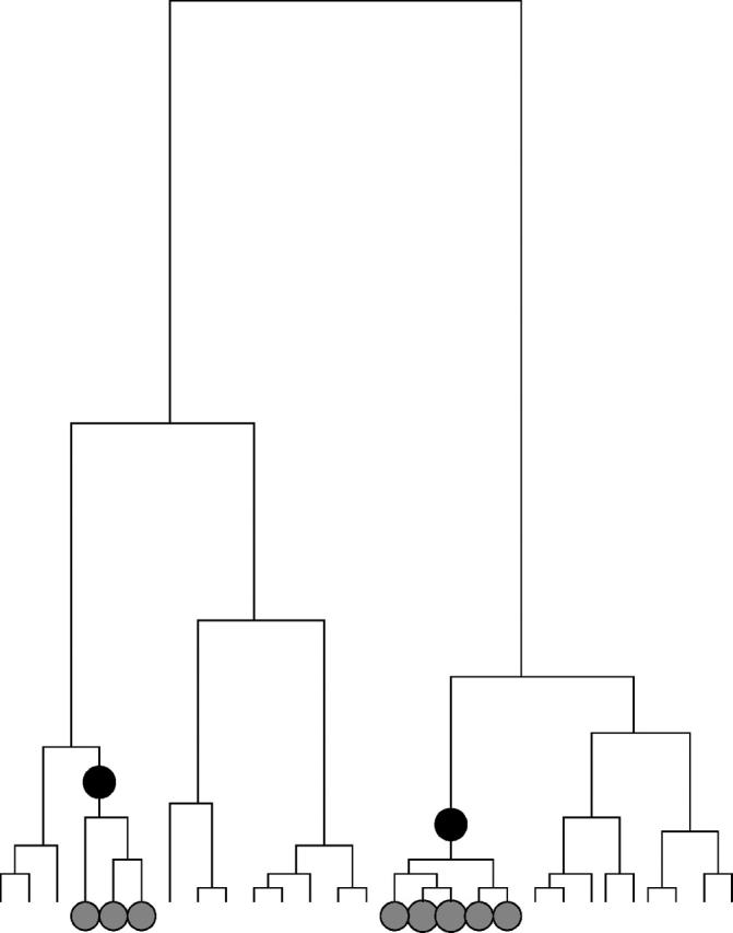
Hypothetical example of a coalescent genealogy for a sample of 28 chromosomes, at the locus of a disease susceptibility gene. Each tip at the bottom of the tree represents a sampled chromosome; the lines indicate the ancestral relationships among the chromosomes. The two solid circles on the tree represent two independent mutation events producing susceptibility variants. These are inherited by the chromosomes marked with hatched circles. Individuals carrying those chromosomes will be at increased risk of disease. This means that there will be a tendency for chromosomes from affected individuals to cluster together on the tree, in two mutation-carrying clades. The degree of clustering depends in part on the penetrance of the mutation.
Traditional methods of association mapping work by testing for association between the phenotype status and alleles at linked marker loci (or with haplotypes). In effect, association at a marker indicates that in the neighborhood of this marker, chromosomes from affected individuals are more closely related to one another than by random. Fundamentally, the marker data are informative because they provide indirect information about the ancestry of unobserved disease variants. Detecting association at noncausative SNPs implies that case chromosomes are nonrandomly clustered on the tree.
In fact, unless we have the actual disease variants in our marker set, the best information that we could possibly get about association is to know the full coalescent genealogy of our sample at that position. If we knew this, the marker genotypes would provide no extra information; all the information about association is contained in the genealogy. Hence, our approach is to use the marker information to learn as much as we can about the coalescent genealogy of the sample at different points along the chromosome. Our statistical inference for association mapping or fine mapping will be based on this. In what follows, we outline our approach of using marker data to estimate the unknown coalescent ancestry of a sample and describe how this information can be used to perform inference. Unlike in previous mapping methods (e.g., Morris et al. 2002), we aim to reconstruct the genealogy of the entire sample and not just the genealogy of cases. This extension allows us to extract substantially more information from the data and enables significance testing.
Performing inference:
We start by developing some notation. Consider a sample of n haplotypes from n/2 unrelated individuals. The phenotype of individual i is φ_i_, and Φ represents the vector of phenotype data for the full sample of n/2 individuals. The phenotypes might be qualitative (e.g., affected/unaffected) or quantitative measurements.
Each individual is genotyped at a series of marker loci from one or more genomic regions (or in the future possibly from genome-wide scans). Let G denote the multidimensional vector of haplotype data—i.e., the genotypes for n haplotypes at L loci (possibly with missing data). Let X be the set of possible locations of the QTL or disease susceptibility gene and let x ∈ X represent its (unknown) position. Our approach is to scan sequentially across the regions containing genotype data, considering many possible positions for x. A natural measure of support for the presence of a disease mutation at position x is given by the likelihood ratio (LR),
 |
1 |
|---|
where _L_A and _L_0 represent likelihoods under the alternative model (disease mutation at x) and null hypothesis (no disease mutation in the region), respectively. _P̂_alt and _P̂_0 are the vectors of penetrance parameters under the alternative and null hypotheses, respectively, that maximize the likelihoods. Large values of the likelihood ratio indicate that the null hypothesis should be rejected. Specific models to calculate these likelihoods are described below (see Equations 7 and 8).
We also want to estimate the location of disease mutations. For this purpose it is convenient to adopt a Bayesian framework, as this makes it more straightforward to account for the various sources of uncertainty in a coherent way (Morris et al. 2000, 2002; Liu et al. 2001). The posterior probability that a disease mutation is at x is then
 |
2 |
|---|
 |
3 |
|---|
where Pr(x) gives the prior probability that the disease locus is at x. Pr(x) will normally be set uniform across the genotyped regions, but this prior can easily be modified to take advantage of prior genomic information if desired (see discussion in Rannala and Reeve 2001; Morris et al. 2002).
To evaluate expressions (1) and (2), we need to compute Pr(Φ, G|x). To do so, we introduce the notation Tx, to represent the (unknown) coalescent genealogy of the sample at x. Tx records both the topology of the ancestral relationships among the sampled chromosomes and the times at each internal node. Then
 |
4 |
|---|
where the integral is evaluated over all possible trees. We now make the following approximations: (i) Pr(Tx|x) ≈ Pr(Tx) and (ii) Pr(G|Φ, x, Tx) ≈ Pr(G|Tx). The first approximation implies that in the absence of the phenotype data, the tree topology itself contains no information about the location of the disease mutation. Thus, we ignore the possible impact of selection and over-ascertainment of affected individuals in changing the distribution of branch times at the disease locus. Our expectation is that the data will be strong enough to overcome minor misspecification of the model in this respect (this was the experience of Morris et al. 2002, in a similar situation). The second approximation is a good assumption if the active disease mutation is not actually in our marker set and if mutations at different positions occur independently. We can then write

and since Pr(G|Tx)Pr(Tx) = Pr(Tx|G)Pr(G) we obtain
 |
5 |
|---|
Expression (5) consists of two parts. Pr(Φ|x, Tx) is the probability of the phenotype data given the tree at x. To compute this, we specify a disease model and then integrate over the possible branch locations of disease mutations in the tree (see below for details). Pr(Tx|G) refers to the posterior density of trees given the marker data and a population genetic model to be specified; the next section outlines our approach to drawing Monte Carlo samples from this density.
In summary, our approach is to scan sequentially across the region(s) of interest, considering a dense set of possible positions of the disease location x. At each position x, we sample M trees denoted T m x from the posterior distribution of trees. For Bayesian inference of location, we apply Equation 2 to estimate the posterior density Pr(x|Φ, G) at x by computing
 |
6 |
|---|
where {_y_1, … , yY} denote a series of Y trial values of x spaced across the region of interest. We will occasionally refer to the numerator of Equation 6, divided by Pr(x), as the “average posterior likelihood” at x. For significance testing at x, we maximize
 |
7 |
|---|
and
 |
8 |
|---|
with respect to _P̂_alt and _P̂_0. See below for details about how these probabilities are computed.
Sampling from the genealogy, Tx:
To perform these calculations, it is necessary to sample from the posterior density, Tx|G (loosely speaking, we wish to draw from the set of coalescent genealogies that are consistent with the genotype data). We adopt a fairly standard population genetic model, namely the neutral coalescent with recombination (i.e., the ARG; Nordborg 2001). Our current implementation assumes constant population size.
A number of recent studies have aimed to perform full-likelihood or Bayesian inference under the ARG (Griffiths and Marjoram 1996; Kuhner et al. 2000; Nielsen 2000; Fearnhead and Donnelly 2001; Larribe et al. 2002; reviewed by Stephens 2001). The experience of these earlier studies indicates that this is a technically challenging problem, and that existing methods tend to perform well only for quite small data sets (e.g., Wall 2000; Fearnhead and Donnelly 2001). Therefore, we have decided to perform inference under a simpler, local approximation to the ARG, reasoning that this might allow accurate inference for much larger data sets. Our implementation applies Markov chain Monte Carlo (MCMC) techniques (see appendix A).
In our approximation, we aim to reconstruct the coalescent tree only at a single “focal point” x, although we use the full genotype data from the entire region, as all of this is potentially informative about the tree at that focal point. Consider two chromosomes that have a very recent common ancestor (at the focal point). These chromosomes will normally both inherit a large region of chromosome around the focal point, uninterrupted by recombination, from that one common ancestor. Then consider a more distant ancestor that the two chromosomes share with a third chromosome in the sample. It is likely that the region around the focal point shared by the three chromosomes is smaller. In our representation of the genealogy, we store the topology at the focal point, along with the extent of sequence at each node that is ancestral to at least one of the sampled chromosomes without recombination (Figure 3).
An example of this is provided in Figure 4. Each tip of the tree records the full sequence (across the entire region) of one observed haplotype. Then, moving up the tree, as the result of a recombination event a part of the sequence may split off and evolve on a different branch of the ARG. When this happens, the amount of sequence that is coevolving with the focal point is reduced. The length of the sequence fragment that coevolves with the focal point can increase during a coalescent event, as the sequence in the resulting node is the union of the two coalescing sequences. In other words, the amount of sequence surrounding the focal point shrinks when a recombination event occurs and may increase at a coalescent event. A marker is retained up to a particular node as long as there is at least one lineage leading to this node in which that SNP is not separated from the focal point by recombination. We do not model coalescent events in the ARG where only one of the two lines carries the focal point. Therefore, the sequence at internal nodes will always consist of one contiguous fragment of sequence.
Figure 4.—

Example of an ancestral genealogy as modeled by our tree-building algorithm. The ancestry of a single focal point (designated F) as inferred from three biallelic markers is shown (alleles are shown as 0 and 1). Branches with recombination events on them are depicted as red lines, showing at the tip of the arrow the part of the sequence that evolves on a different genealogy. As can be seen at the coalescent event at time _t_4, if no recombination occurs on either branch, the entire sequence is transmitted along a branch and coalesces, generating a full-length sequence. If on the other hand a recombination event occurs, the amount of sequence that reaches the coalescent event is reduced (indicated by the dashes). If this reduction occurs on only one of the two branches, the sequence can be restored from the information on the other branch (as at time _t_3). But if recombination events occur on both branches, the length of the sequence is reduced (_t_2).
Our MCMC implementation stores the tree topology, node times, and the ancestral sequence at each node. We assume a finite sites mutation model for the markers that are retained on each branch. (This rather simplistic model is far more computationally convenient than more realistic alternatives.) At some points, sequence is introduced into the genealogy through recombination events. We approximate the probability for the introduced sequence by assuming a simple Markov model on the basis of the allele frequencies in the sample (similar approximations have been used previously by McPeek and Strahs 1999; Morris et al. 2000; Liu et al. 2001; Morris et al. 2002). The population recombination rate ρ and the mutation rate θ are generally unknown in advance and are estimated from the data within the MCMC scheme, assuming uniform rates along the sequence. A more precise specification of the model and algorithms is provided in appendix A.
Overall, our model is similar to those of earlier approaches such as the haplotype-sharing model of McPeek and Strahs (1999) and the coalescent model of Morris et al. (2002). However, we focus on chromosomal sharing backward in time, rather than on decay of sharing from an ancestral haplotype. In part, this reflects our shift away from modeling only affected chromosomes to modeling the tree for all chromosomes. The representation used by those earlier studies means that they potentially have to sum over possible ancestral genotypes at sites far away from the focal point x, which are not ancestral to any of the sampled chromosomes and about which there is therefore no information. Storing all this extra information is likely to be detrimental in an MCMC scheme, as it presumably impedes rearrangements of the topology. Thus, we believe that our representation can potentially improve both MCMC mixing and the computational burden involved in each update. Indeed, if one wished to perform inference across an infinitely long chromosomal region, the total amount of sequence stored at the ancestral nodes in our representation would be finite, while that in the earlier methods would not.
A more fundamental difference is that, unlike most of the previous model-based approaches to this problem, our genealogical reconstruction is independent of the phenotype data. There are trade-offs in choosing to frame the problem in this way, as follows. When the alternative model is true, the phenotype data contain some information about the topology that could help to guide the search through tree space. In contrast, our procedure weights the trees after sampling them from Pr(Tx|G) according to how consistent they are with the phenotype data (Equations 6 and 7), ignoring additional information from the phenotype data. However, tackling the problem in this way makes it far easier to assess significance, because we know that under the null the phenotypes are randomly distributed among tips of the tree. It also means that we can calculate posterior densities for multiple disease models using a single MCMC run.
Modeling the phenotypes:
To compute expressions (6) and (7), we use the following model to evaluate Pr(Φ|x, Tx). At the unobserved disease locus, let A denote the genotype at the root of the tree Tx. We assume that genotype A mutates to genotype a at rate ν/2 per unit time, independently on each branch. We further assume that alleles in state a do not undergo further mutation.
Next, we need to define a model for the genotype-phenotype relationship for each of the three diploid genotypes at the susceptibility locus: namely, Pr(φ|AA), Pr(φ|Aa), and Pr(φ|aa), where φ refers to a particular phenotype value (e.g., affected/unaffected or a quantitative measure). For a binary trait, these three probabilities denote simply the genotypic penetrances: e.g., Pr(Affected|AA). In practice, the situation is often complicated by the fact that the sampled individuals may not be randomly ascertained. In that case, the estimated “penetrances” really correspond to Pr(φ|AA, S), Pr(φ|Aa, S), and Pr(φ|aa, S), where S refers to some sampling scheme (e.g., choosing equal numbers of cases and controls).
In the algorithm presented here, we assume that the affection status of the two chromosomes in an individual can be treated independently from each other and from the frequency of the disease mutation: i.e., PA(φ) is the probability that a chromosome with genotype A comes from an individual with phenotype φ, and analogously for Pa(φ). In the binary situation, this model has two independent parameters: PA(1) = 1 − PA(0) and Pa(1) = 1 − Pa(0). In this case the ratio PA(φ)/Pa(φ) corresponds directly to the relative risk of allele A, conditional on the sampling scheme. As another example, for a normally distributed trait, PA(φ) and Pa(φ) are the densities of two normal distributions at φ and would be characterized by mean and variance parameters. Note that most values of PA(φ) and Pa(φ) do not correspond to a single genetic model that exists as the mapping from (PA(φ), Pa(φ)) to (Pr(φ|AA), Pr(φ|Aa), Pr(φ|aa)) is dependent on the frequency of the disease mutation. Nevertheless, this factorization of the penetrance parameters is computationally convenient and allows for an efficient analysis of Tx.
Of course, it is not known in advance which chromosomes are A and which are a, so we compute the likelihood of the phenotype data by summing over the possible arrangements of mutations at the disease locus. Under the alternative hypothesis, most arrangements of mutations will be relatively unsupported by the data, while branches leading to clusters of affected chromosomes will have high support for containing mutations. Let M record which branches of the tree contain disease mutations and γ ⊂ {1, … , n} be the set of chromosomes that carry a disease mutation according to M (i.e., the descendants of M) and let β be the set of chromosomes that do not carry a mutation, i.e., β = {1, … , n}\γ. Then we calculate
 |
9 |
|---|
For a case-control data set this can be written as

where n _i_d and n _i_h count the number of _i_-type chromosomes (where i ∈ {A, a}) from affected and healthy individuals, respectively. Equation 9 can be evaluated efficiently using a peeling algorithm (Felsenstein 1981). The details of this algorithm are provided in appendix B. Calculations for general diploid penetrance models are much more computationally intensive, and we will present those elsewhere.
For our Bayesian analysis, we take the prior for the parameters governing PA(φ) and Pa(φ) to be uniform and independent on a bounded set Δ̃ and average the likelihoods over this prior. By allowing any possible order for the penetrances under the alternative model, we allow for the possibility that the ancestral allele may actually be the high-risk allele, as observed at some human disease loci, including ApoE (Fullerton et al. 2000).
For significance testing, we test the null hypothesis that PA(φ) = Pa(φ) compared to the alternative model where the parameters governing PA(φ) and Pa(φ) can take on any values independently. Standard theory suggests that twice the log-likelihood ratio of the alternative model, compared to the null, should be asymptotically distributed as χ2 random values with d d.f., where d is the number of extra parameters in the alternative model compared with the null. Thus, for case-control studies our formulation suggests that twice the log-likelihood ratio should have a χ21 distribution. In fact, simulations that we have done (results not shown) indicate that this assumption is somewhat conservative.
Finally, it remains to determine the mutation rate, ν, at the unobserved disease locus. It seems unlikely that much information about ν will be in the data; hence we prefer to set it to a plausible value, a priori. For a similar model, Pritchard (2001) argued that the most biologically plausible values for this parameter are in the range of ∼0.1–1.0, corresponding to low and moderate levels of allelic heterogeneity, respectively.
Multiple testing:
Typically, association-mapping studies consist of large numbers of statistical tests. To account for this, it is common practice to report a _P_-value that measures the significance of the largest departure from the null hypothesis anywhere in the data set. The simplest approach is to apply a Bonferroni correction (i.e., multiplying the _P_-value by the number of tests), but this tends to be unnecessarily conservative because the association tests at neighboring positions are correlated.
A more appealing solution is to use randomization techniques to obtain an empirical overall _P_-value (cf. McIntyre et al. 2000). The basic idea is to hold all the genotype data constant and randomly permute the phenotype labels. For each permuted set, the tests of association are repeated, and the smallest _P_-value for that set is recorded. Then the experiment-wide significance of an observed P_-value pi is estimated by the fraction of random data sets whose smallest value is ≤_pi.
The latter procedure is practical only if the test of association is computationally fast. For the method proposed in this article, the inference of ancestries is independent of phenotypes. Therefore, the trees need to be generated only once in this scheme and the sampled trees are stored in computer memory. Then, the likelihood calculations can be performed on these trees using both the real and randomized phenotype data to obtain the appropriate empirical distribution.
For a whole-genome scan, a permutation test with the proposed peeling strategy is rather daunting. Performing the peeling analysis for 1000 permutations on one tree of 100 cases and 100 controls takes ∼6 min on a modern desktop machine. Thus, a whole-genome permutation test with one focal point every 50 kb, 100 trees per focal point, and a penetrance grid of 19 × 19 values would take ∼750,000 processor hours.
A rather different solution for genome-wide scans of association may be to apply the false discovery rate criterion, as this tends to be robust to local correlation when there are enough independent data (Benjamini and Hochberg 1995; Sabatti et al. 2003).
Unknown haplotype phase:
Our current implementation assumes that the individual genotype data can be resolved into haplotypes. However, in many current studies, haplotypes are not experimentally determined and must instead be estimated by statistical methods. In principle, it would be natural to update the unknown haplotype phase within our MCMC coalescent framework described below (Lu et al. 2003; Morris et al. 2003). By doing so, we would properly account for the impact of haplotype uncertainty on the analysis. In fact, Morris et al. (2004) concluded that doing so increased the accuracy of their fine-mapping algorithm (compared to the answers obtained after estimating haplotypes via a rather simple EM procedure). However, it is already a difficult problem to sample adequately from the posterior distribution of trees given known haplotypes and it is unclear to us that the added burden of estimating haplotypes within the MCMC scheme represents a sensible trade-off. Therefore, we currently use point estimates of the haplotypes obtained from PHASE 2.0 (Stephens et al. 2001; Stephens and Donnelly 2003). We also currently use PHASE to impute missing genotypes.
False positives due to population structure:
It has long been known that case-control studies of association are susceptible to high type 1 error rates when the samples are drawn from structured or admixed populations (Lander and Schork 1994). Therefore, we advise using unlinked markers to detect problems of population structure (Pritchard and Rosenberg 1999), prior to using the association-mapping methods presented here.
When population structure is problematic, there are two types of methods that aim to correct for it: genomic control (Devlin and Roeder 1999) and structured association (Pritchard et al. 2000; Satten et al. 2001). It seems likely that some form of genomic control correction might apply to our new tests, but it is not clear to us how to obtain this correction theoretically. It should be possible to obtain robust _P_-values using the structured association approach roughly as follows. First, one would apply a clustering method to the unlinked markers to estimate the ancestry of the sampled individuals (Pritchard et al. 2000; Satten et al. 2001) and the phenotype frequencies across subpopulations. Then, the phenotype labels could be randomly permuted across individuals while preserving the overall phenotype frequencies within subpopulations. As before, the test statistic of interest would be computed for each permutation.
SNP ascertainment and heterogeneous recombination rates:
In the MCMC algorithm described above, and more fully in appendix A, we assume—for convenience—that mutation at the markers can be described using a standard finite sites mutation model with mutation parameter θ. However, in practice, we aim to apply our method to SNPs: markers for which the mutation rate per site is likely to be very low, but that have been specifically ascertained as polymorphic. Hence, our estimate of θ should not be viewed as an estimate of the neutral mutation rate; it is more likely to be roughly the inverse of the expected tree length (if there has usually been one mutation per SNP in the history of the sample). Moreover, the fact that SNPs are often ascertained to have intermediate frequency and that we overestimate θ may lead to some distortion in the estimated branch lengths. However, we anticipate that most of the information about the presence of disease variation will come from the degree to which case and control chromosomes cluster on the tree, so bias in the branch length estimates may not have a serious impact on inferences about the location of disease variation. The next section provides results supporting this view.
Another factor not considered in our current implementation is the possibility of variable recombination rate (e.g., Jeffreys et al. 2001). Since recombination rates appear to vary considerably over quite fine scales, this is probably an important biological feature to include in analysis. One route forward would be for us to estimate separate recombination parameters in each intermarker interval, within the MCMC scheme (perhaps correlated across neighboring intervals). It is unclear how much this would add to the computational burden of convergence and mixing. In the short term, it would be possible to use a separate computational method to estimate these rates prior to analysis with local approximation to the ancestral recombination graph (LATAG; e.g., using Li and Stephens 2003) and to modify the input file to reflect the estimated genetic distances.
Software:
The algorithms presented here have been implemented in a program called LATAG. The program is available on request from S. Zöllner.
TESTING AND APPLICATIONS: SIMULATED DATA
To provide a systematic assessment of our algorithm we simulated 50 data sets, each representing a fine-mapping study or a test for association within a candidate region. Each data set consists of 30 diploid cases and 30 diploid controls that have been genotyped for a set of markers across a region of 1 cM. Our model corresponds to a scenario of a complex disease locus with relatively large penetrance differences (since the sample sizes are small) and with moderate allelic heterogeneity at the disease locus.
The data sets were generated as follows. We simulated the ARG, assuming a constant population size of 10,000 diploid individuals and a uniform recombination rate. On the branches of this ARG, mutations occurred as a Poisson process according to the infinite sites model. The mutation rate was set so that in typical realizations there would be 45–65 markers with minor allele frequency >0.1 across the 1-cM region. The position of the disease locus xs was drawn from a uniform distribution across the region. Mutation events at the disease locus were simulated on the tree at that location at rate 1 per unit branch length (in coalescent time), with no back mutations (cf. Pritchard 2001). This process determines whether each chromosome does, or does not, carry a disease mutation. We required that the total frequency of mutation-bearing chromosomes be in the range 0.1–0.2, and if it was not, then we simulated a new set of disease mutations at the same location. This procedure generated a total of 10–25 disease mutations across the entire population, although many of the mutations were redundant or at low frequency.
To assign phenotypes, we used the following penetrances: a homozygote wild type showed the disease phenotype with probability _P_hw = 0.05, a heterozygous genotype showed it with probability _P_he = 0.1, and a homozygous mutant showed it with probability _P_hm = 0.8. According to these penetrances, we then created 30 case and 30 control individuals by sampling without replacement from the simulated population of 20,000 chromosomes, as follows. Let n be the remaining number of wild-type chromosomes in the population and m be the remaining number of mutant chromosomes in the population. Then the next case individual was homozygous for the mutation with probability (_P_hm · m · (m − 1)) · (_P_hm · m · (m − 1) + 2 · _P_he · m · n + _P_hw · n · (n − 1))−1, heterozygous with probability (2 · _P_he · m · n) · (_P_hm · m · (m − 1) + 2 · _P_he · m · n + _P_hw · n · (n − 1))−1, and otherwise homozygous for the mutant allele. The diplotypes for each case were then created by sampling the corresponding number of mutant or wild-type chromosomes. Control individuals were generated analogously. Across the 50 replicates, we found that 10–33 of the 60 case chromosomes and 0–9 of the control chromosomes carried a disease mutation.
As might be expected for the simulation of a complex disease, not all of the simulated data sets carried much information about the presence of genetic variation influencing the phenotype. For instance, in 22 of the generated data sets, the highest single-point association signal among the generated markers, calculated as Pearson's χ2, is <6.5.
We analyzed each simulated data set by considering 50 focal points _x_1, … , x_50, spaced equally across the 1-cM region. For each point xi we used LATAG to draw 50 trees from the distribution Pr_T x i|G, x i. To ensure convergence of the MCMC, we used a burn-in period of 2.5 × 10⁶ iterations for _x_1. As the tree at location xi is a good starting guess for trees of the adjacent tree at xi+1 we used a burn-in of 0.5 × 10⁶ iterations for _x_2, … , xk. We sampled each set of trees T_1_x i, … , T_50_x i using a thinning interval of 10,000 steps and estimated Pr(Φ, G|xi) according to (6) and (B2) without assuming any prior information about the location of disease mutations. We found that the mean was somewhat unstable due to occasional large outliers and therefore substituted the median for the average in (6). To evaluate (B2) we summed over a grid of penetrances Δ̃ = {0.05, 0.1, … , 0.95} × {0.05, 0.1, … , 0.95}, setting the disease mutation rate ν to 1.0. We calculated the posterior probability at each locus xi by evaluating
In addition, we recorded the point estimate for the location of the disease mutation as the xi with the highest posterior probability. The running time for each data set was ∼5 hr on a 2.4-GHz processor with 512 K memory.
For comparison, we also analyzed each data set with DHSMAP-map 2.0 using the standard settings suggested in the program package. This program generated point estimates for the locus of disease mutation and two 95% confidence intervals: the first assuming a star-like phylogeny among cases, and the second using a correction to account for the additional correlation among cases that results from relatedness.
Significance tests were performed by two methods. First we calculated
 |
10 |
|---|
and calculated the likelihood ratio according to (1),

with _L_0 = 0.5120. We assigned pointwise significance to this ratio by assuming that 2 ln(LR) is χ2-distributed with 1 d.f. (Other simulations that we have done indicate that this assumption is somewhat conservative; results not shown.) To estimate global significance, we permuted case and control status among the 60 individuals 1000 times, recalculated Lm for each permutation (using the original trees obtained from the data), and counted the number of permutations that showed a higher Lm than the original data set anywhere in the region. The permutation procedure corrects for multiple testing across the region and does not rely on the predicted distribution of the likelihood ratio.
For comparison we assessed the performance of single-point association analysis by calculating the association of each observed marker in a 2 × 2-contingency table with a χ2-statistic and recorded the χ2 of the marker with the highest value. We assigned significance to this test statistic in two ways: first, on the basis of the χ2-distribution with 1 d.f., and second, by performing 1000 permutations of phenotypes among the 60 individuals and counting the number of permutations in which the highest observed χ2 was higher than that observed in the sample.
To assess convergence, we then repeated the analysis of each data set an additional four times and compared the estimated posterior distributions to assess the convergence of the MCMC and the variability in estimation. We calculated the overlap of two credible intervals _C_1 and _C_2 obtained from multiple MCMC analyses of the same data set as
where |I| is the length of interval I.
RESULTS
Assessing convergence:
An important issue for MCMC applications is to check the convergence of the Markov chain, since poor convergence or poor mixing can lead to unreliable results. While numerous methods exist to diagnose MCMC performance (Gammerman 1997), the most direct approach is to compare the results from multiple MCMC runs. If the Markov chain performs well, and the samples drawn from the posterior are sufficiently large, then different runs will produce similar results. (Conversely, good performance by this criterion does not absolutely guarantee that the Markov chain is working well, but it is certainly encouraging.)
To assess the convergence of the LATAG algorithm, we performed five runs for each of the 50 simulated data sets. For our simulated data sets we found that on average, pairs of 50% credible intervals overlapped by 75% and pairs of 95% credible intervals overlapped by 96%.
As a second method of evaluating the convergence of the MCMC, we compared the point estimates for the location of disease mutation between the different runs. The average distance between two point estimates on the same data set is 184 kb. This number includes data sets where there is very little information about the locus of disease mutation. Figure 5 displays the point estimates for across independent runs, indicating that for most data sets all five runs produce a similar estimate. Further inspection of the results in Figure 5 indicates that in most cases where there is substantial variation across runs, this is because the posterior distribution is relatively flat across the entire region. Some of the data sets contain very little information about the presence or location of disease mutations, and so small random fluctuations in the estimation can shift the peak from one part of the region to another. To further quantify this observation, we computed the correlation between the average pairwise difference of the point estimates with the average posterior likelihood at the point estimate for each data set. We observed that these were strongly negatively correlated (correlation coefficient = −0.29). The higher the signal that is present in the data (expressed in posterior probability), the smaller the difference is between the point estimates.
Figure 5.—

Point estimates of the locus of disease mutation for five independent MCMC analyses of each of 50 simulated data sets. The data sets are ordered from left to right by the median point estimate across the five replicates. The shading of the point indicates the strength of the signal at the point estimate: darker points indicate stronger signals in the data. Open points correspond to estimates where the average posterior likelihood is <1.2-fold higher than the expected posterior likelihood in the absence of disease mutations, shaded triangles correspond to estimates that are 1.2–12-fold higher than the background, and solid circles correspond to estimates that are >12-fold higher than background.
In summary, when the data sets contained a strong signal, the concordance between individual runs was quite high, indicating good convergence. On the other hand, when the information about location was weak, random variation across runs meant that the point estimates sometimes varied considerably. In such cases, longer runs would be needed to obtain really accurate estimates. For analyzing real data, it is certainly important to use multiple LATAG runs to ensure the robustness of the results.
Point estimates of location:
The mode of the posterior distribution is a natural “best guess” for the location of the disease variation. To assess the accuracy of this estimate, we calculated the distance between this point estimate and the real locus of the disease mutation for each simulated data set. Overall, we observed an average error of 0.19 cM with a standard deviation of 0.23 cM. To evaluate this result, we compared it to the accuracy of two other point estimators. As a naive estimator, we chose the position of the marker that has the highest level of association with the phenotype, measured using the Pearson χ2 statistic. This choice is based on the observation that, on average, LD declines with distance. As an example of an estimator provided by a multipoint method, we analyzed the prediction generated by DHSMAP.
We found that the average distance between the disease locus and the SNP with the highest χ2 was 0.25 cM (standard deviation 0.26 cM) and the distance to the DHSMAP point estimate was 0.27 cM (standard deviation 0.25 cM). The cumulative distributions of the error in estimation are displayed in Figure 6. The estimate generated by LATAG is most likely to be close to the real locus of disease mutation. For instance, in 54% of all simulations, the LATAG estimate is within 0.1 cM of the real locus, while the naive estimate is within 0.1 cM in 44% of all cases and DHSMAP is in the same range in 30% of our simulated data sets.
Figure 6.—

Cumulative distribution of distances (in centimorgans) between the locus of disease mutation and point estimates from three different methods. From top to bottom, the three estimates are obtained from LATAG, DHSMAP, and from the location of the SNP with the highest single-point χ2-value in a test for association.
Coverage of credible intervals:
A major advantage of using model-based methods to estimate disease location is that they can also provide a measure of the uncertainty of an estimate. To assess the accuracy of the estimated uncertainty for LATAG, we generated credible intervals of different sizes, ranging from 10 to 90%, on the basis of the posterior distribution for each data set. Figure 7 plots the number of data sets for which the disease mutation is located within each size credible interval and compares those numbers to the expected values. There is good accordance between the values, although it appears that for low and intermediate confidence levels the constructed intervals are somewhat conservative and that the posterior distribution generated by LATAG slightly overestimates the uncertainty. The high uncertainty about the location of the disease mutation is reflected in the average size of the confidence intervals, which range from 0.06 cM for the 10% C.I. to 0.85 cM for the 90% C.I.
Figure 7.—

Coverage accuracy of the credible intervals obtained by LATAG. We constructed credible intervals of different sizes, ranging from 10 to 90% (_x_-axis). The _y_-axis shows the number of data sets (out of 50) for which the credible interval contained the true location of the disease gene. The blue bars (number observed) are generally slightly higher than the purple bars (number expected if the coverage is correct), suggesting that our credible intervals may be slightly conservative.
For comparison, we also looked at the 95% confidence intervals that are generated by DHSMAP. Those intervals are considerably shorter than the intervals obtained from LATAG, at an average length of 0.37 cM for intervals obtained using the correction for pairwise correlation and 0.15 cM without that correction. But for both models the confidence intervals were too narrow, with 48 and 18%, respectively, of intervals containing the true disease locus (cf. Morris et al. 2002). In summary, LATAG seems to provide credible regions that are fairly well calibrated or perhaps slightly conservative.
Hypothesis testing:
To gauge the power of LATAG in a test for association, we assessed for each data set whether we could detect the simulated region as a region harboring a disease mutation. To do this, we calculated the likelihood ratio at each focal point according to Equation 1 and considered the maximal LR that we observed among all focal points as the evidence for association. For comparison, we also tested each SNP for association with the phenotype, using a standard Pearson χ2-test. We obtained an average maximum value of twice the log-likelihood ratio of 5.8 and an average maximum SNP-based χ2 of 8.5. In 88% of the simulations, the χ2-test generated a more significant single-point _P_-value.
However, because the extent of multiple testing may be different for the two methods, this is not exactly the right comparison. The LATAG analysis consists of 50 tests, many of which are highly correlated, because the trees may differ little from one focal point to the next. The SNP-based test consists of about the same number of tests (one for each marker), and the correlation between tests depends on the LD between the markers. Therefore, a simple Bonferroni correction is too conservative for both test statistics. To perform tests that take the dependence structure in the data into account, we obtained _P_-values for each of the two test statistics by permutation (see Simulation methods). We observed that correcting for multiple tests has a strong impact on the signal of the single-point analysis. For 24% of the data sets, the single-point analysis produced a region-wide _P_-value <0.05, while in 30% of the data sets LATAG produced a _P_-value <0.05. Furthermore, the two tests do not always detect the same data sets: one-third of all the data sets that showed a significant single-point score did not have a significant signal with LATAG, while 45% of all disease loci that were detected with LATAG were not detected with the single-point analysis (Figure 8). Hence, although LATAG appears to be more powerful on average, there may be some value in performing SNP-based tests of association as well as that approach may detect some loci that would not be detected by LATAG.
Figure 8.—

Comparison of the ability of LATAG (_x_-axis) and a SNP-based χ2-test (_y_-axis) to detect disease-causing loci in a test for association. Each point corresponds to one of the 50 simulated data sets and plots the most significant _P_-values obtained for that data set using each method, corrected for multiple testing within the region. The dotted lines depict the P = 0.05 cutoffs and the diagonal line plots the regression line through the log-log-transformed data.
TESTING AND APPLICATIONS: REAL DATA
To further illustrate our method we report analyses of two sets of case-control data. One data set was used to map the gene responsible for cystic fibrosis, a simple recessive disorder (Kerem et al. 1989), while the other data set is from a positional cloning study of a complex disease, type 2 diabetes (Horikawa et al. 2000).
Example application 1:
Cystic fibrosis:
The cystic fibrosis (CF) data set used by Kerem et al. (1989) to map the CFTR locus has been used to evaluate several previous fine-mapping procedures, thus allowing an easy comparison between LATAG and other multipoint methods. The data set was generated to find the gene responsible for CF, a fully penetrant recessive disorder with an incidence of 1/2500 in Caucasians. Many different disease-causing mutations have been observed at the CFTR locus, but the most common mutation, ΔF508, is at quite high frequency, accounting for 66% of all mutant chromosomes.
The data set consists of 23 RFLPs distributed over 1.8 Mb; these were genotyped in 47 affected individuals. In addition, 92 control haplotypes were obtained by sampling the nontransmitted parental chromosomes. High levels of association were observed for almost all markers in the region; the marker with the highest single-point association (χ2 = 63) is located at 870 kb from the left-hand end of the region. The ΔF508 mutation is at 885 kb and is present in 62 of the 94 case chromosomes.
We ran 10 independent runs of the Markov chain, estimating the average posterior likelihood at each of 50 evenly distributed points across the region. Each run had a burn-in of 2.5 × 10⁶ steps for the first focal point and 106 steps for each following focal point. In each run, we sampled 50 trees at each focal point, with a thinning interval of 10,000 steps. The runs took 8 hr each on a Pentium III processor. For each tree Ti, we calculated P(Φ|Ti, x) with the peeling algorithm. As the resulting posterior likelihoods seemed to be heavily dependent on a few outliers, we estimated the likelihood P(x|Φ, G) at each position x by taking the median of the likelihoods P(Φ|Ti, x) instead of the average suggested by theory. As before, we used the posterior mode as our point estimate for location. Missing data were imputed using PHASE 2.0 (Stephens et al. 2001).
Results:
To provide a simple check of convergence, Figure 9 shows the results from the 10 independent analyses of the CF data set. As can be seen, all 10 runs have modes in the same region and yield the same conclusion about the location of the causative variation.
Figure 9.—

Repeatability across runs. Average posterior likelihoods for 10 independent LATAG analyses of the CF data set are shown. For the location of the disease locus and the resulting posterior credible region refer to Figure 10.
Figure 10 summarizes our results across the 10 runs. The posterior distribution is sharply peaked at 867 kb, near the true location of ΔF508 (which is at 885 kb). The 95% credible interval is rather narrow, extending from 814 to 920 kb. Even though several markers with little association to the trait are in the vicinity of the deletion (Figure 10), the LATAG estimate is quite accurate. It is useful to compare our results to those obtained by other multipoint methods (see Table 1, modified from Morris et al. 2002). For this data set, most of the highest single-point χ2 values lie to the left of the true location of ΔF508, and so most of the methods err to the left, with some of the earliest methods (Terwilliger 1995) actually excluding the true location from the confidence interval. Note that the LATAG estimate is closer to the true location, and that the 95% credibility region is narrower than that obtained by any of the previous methods.
Figure 10.—

Average posterior likelihoods generated by LATAG for the CF data set (Kerem et al. 1989). The dots depict the association signals of the individual markers as χ2-statistics (see scale on the right). We display the likelihoods here because the posterior density is extremely peaked, with 95% of its mass inside the box marked by the dashed lines.
TABLE 1.
Estimates of locations of the CF-causing allele, as taken from Morris et al. (2002)
| Method | Estimate | Variability | Comments |
|---|---|---|---|
| Terwilliger (1995) | 770 | 690–870 (99.9% support interval) | |
| McPeek and Strahs (1999) | 950 | 440–1460 (95% confidence interval) | Pairwise correction |
| Morris et al. (2000) | 800 | 610–1070 (95% credible interval) | Pairwise correction |
| Liu et al. (2001) | — | 820–930 (95% credible interval) | |
| Morris et al. (2002) | 850 | 650–1000 (95% credible interval) | |
| LATAG | 867 | 814–920 (95% credible interval) |
To assess the ability of LATAG to detect the CF region by association, we calculated a likelihood ratio according to (1) and obtained 2 ln(LR) = 40. Assuming a χ2-distribution with 1 d.f., this log-likelihood ratio has an associated _P_-value of 3.7 × 10⁻¹⁰. While this is extremely significant, it is less significant than that obtained from simple tests of association with individual SNPs (six of which yield χ2-values >50). This may indicate that our likelihood-ratio test does not fit the χ2-approximation very well, particularly far out in the tail of the distribution, or that our test is slightly less powerful in this extreme setting. Due to the extremely high level of significance, it is infeasible to generate an accurate _P_-value by permutation.
Example application 2:
Calpain-10:
Our second application comes from a positional cloning study that was searching for disease variation underlying type 2 diabetes. Type 2 diabetes is the most common form of diabetes and in developed countries it affects 10–20% of individuals over the age of 45 (Horikawa et al. 2000). This appears to be a highly complex disease, with no gene of major effect, and with environmental factors playing an important role. A linkage study in Mexican Americans localized a susceptibility gene to a region on chromosome 2 containing three genes, RNEPEPL1, CAPN10, and GPR35. A data set that was generated by Horikawa et al. (2000) for positional cloning consists of 85 SNPs distributed over an area of 876 kb. The markers were genotyped in 108 cases and 112 controls. No individual marker shows high association; the marker with the highest LD (χ2 = 9) is located at 121 kb from the left-hand end of the region. The original study also used some additional information from family-sharing patterns that we do not consider here. On the basis of detailed analysis of those data, Horikawa et al. (2000) proposed that a combination of two haplotypes, each consisting of 3 SNPs within the CAPN10 gene, increases the risk of diabetes by two- to fivefold. The three SNPs that make up the haplotype are located at 121, 124, and 134 kb.
We used the PHASE 2.0 algorithm, with recombination in the model (Stephens et al. 2001), to impute the phase information and missing genotypes for both cases and controls. Then we used LATAG to infer the posterior distribution of the location of the disease mutation and a _P_-value for association, as described above. Performing eight independent runs of the MCMC, we generated a total of 800 draws from the posterior distribution P(T|G, x) for each of 50 positions in the sequence. Each run had a burn-in of 5 × 10⁶ steps for the first point and 106 steps for each following point, a thinning interval of 10,000 steps between draws, and took 36 hr on a Pentium III processor.
Results:
Figure 11 plots the estimated posterior distribution for the location of diabetes-associated variation in this region. From this distribution we estimate the position of the disease mutation at 131 kb, at the same location as the SNPs that Horikawa et al. (2000) reported as defining the key haplotypes. However, the posterior distribution is quite wide, with 50% of its mass between 70 and 245 kb. The full 95% credibility region extends between 0 and 660 kb, indicating that we can really exclude only the right-hand end of this region. We would need larger samples to obtain more precision.
Figure 11.—

Posterior distribution for the location of the diabetes-affecting variant(s) in the calpain-10 region (solid line; see scale on the left). The dots represent the association of individual markers with the phenotype (see χ2-scale on the right). The red dots indicate the three markers that define the disease-associated haplotypes reported by Horikawa et al. (2000).
To assess whether we would have detected this region by association, on the basis of this data set, we evaluated (1) and obtained 2 ln(LR) = 6.0 at the posterior mode, corresponding to a single-point _P_-value of 5.3 × 10⁻⁴. When we correct for multiple testing using the simulation procedure, the overall significance level drops to a mildly significant P = 0.02. In contrast, if we assess the significance of the highest observed single-point χ2 by permuting case and control labels, we obtain a nonsignificant _P_-value of 0.11.
Overall, our results are consistent with the conclusion of Horikawa et al. (2000), that CAPN10 is the gene that was responsible for their diabetes linkage signal in this region. However, our analysis cannot exclude GPR35 as the disease gene. As with the original analysis, our strongest signal is in the CAPN10 region, but our overall signal is only modestly significant.
DISCUSSION
We have described a new unified method, LATAG, for association mapping and fine mapping with multipoint data. Our approach, based on a local approximation to the ARG, strikes a compromise between modeling the population genetic processes that produce the data and the need for a model that is computationally tractable for large data sets.
Our association-mapping method is similar in spirit to earlier tree-based methods (e.g., Templeton et al. 1987). However, we take a more probabilistic approach in the sense that we average over the uncertainty in trees and consider an explicit mutation model at the unobserved disease locus. A more fundamental difference is that our tree inference scheme aims to model recombination explicitly, while the earlier methods make the most sense in small regions without evidence for recombination. Moreover, even for estimating the tree within a haplotype block, markers outside the block may contain additional information about that tree. It is typical for there to be at least some LD between haplotype blocks (Daly et al. 2001), and patterns of haplotype sharing across multiple blocks are potentially quite informative about the order of recent coalescent events. In our method, rather than forcing the user to predefine regions of limited recombination, the algorithm “adapts” to the data, in the sense that quite large regions of shared haplotypes may help to resolve recent coalescent events, while much smaller regions (e.g., corresponding to haplotype blocks) may be the relevant scale for reconstructing the topology of the more ancient coalescent events. Hence, we gather information both from mutation and from recombination events to reconstruct the ancestral trees. By doing so, we can detect association even when there is allelic heterogeneity, and we can gain information about low-frequency disease mutations, even using only intermediate-frequency SNPs. Our simulations indicated that LATAG is substantially more powerful than single-point SNP-based tests of association, at least for the scenario considered.
It is also natural to compare LATAG to recent fine-mapping algorithms. One major difference between LATAG and most of the previous coalescent-based algorithms is that LATAG aims to reconstruct the ancestry of all the sampled chromosomes, not just of case chromosomes. By considering the ancestry of all individuals at once, we can deal with more general phenotype models and we can model allelic heterogeneity and incomplete penetrance in a natural way, although including this additional information may increase computation time. This also represents the first multipoint fine-mapping method for quantitative traits. Our approach can also produce penetrance estimates under haploid and diploid models (the latter to be presented elsewhere), although these estimates may not be straightforward to interpret when the ascertainment of samples is not random. We have not focused on this here, but our approach also produces a posterior probability that each chromosome carries a disease mutation. This can be used to guide full resequencing of implicated regions. Including control chromosomes in the tree allows us to make better use of the control data than earlier methods that used just controls to estimate the SNP allele frequencies, as exemplified by the strong performance of our method on the CF data and on the simulated data.
For any model-based approach such as LATAG, it is worth considering the various modeling assumptions and how these might affect the results. In general, it seems that most of the inaccuracies of the model can be overcome by informative data; at worst they might slightly reduce our power and precision (cf. Morris et al. 2002). For instance, the Markov model that we use for LD outside the inherited region is not strictly accurate and might be expected to produce a slight bias toward keeping too much sequence on the tree. Inaccuracies there may explain the tendency toward conservativeness in the coverage of our credible intervals (Figure 7). Similarly, the finite sites model used for SNP mutation, ignoring SNP ascertainment, is clearly inaccurate. However, this model is computationally convenient, and it seems likely that the data should overwhelm deficiencies here; again, that view is supported by the results. Besides, allowing recurrent SNP mutation provides an ad hoc way of allowing for gene conversion, which might otherwise confound our inference.
Another issue is that we ignore the ascertainment of cases and natural selection on the disease variants. These processes are expected to distort the shape of the tree (cases will be more closely related than predicted under the coalescent model). But this distortion effect will be most pronounced when the signal is very strong (e.g., for a recent highly penetrant mutation, as in the CF data). In that case, the data will usually be strong enough to overwhelm the rather weak coalescent prior. In other words, when the coalescent model is furthest from the truth, the data are likely to be very informative and should override the misspecifications of the prior.
At present we also assume that even if there are multiple disease mutations in a region all of these occur at essentially the same position. This may well be a poor assumption. For example, mutations in different exons of a single gene might be many kilobases apart. Neither our method nor any other existing method would handle this well; however, dealing with this issue is surely an important problem for the future.
Full-likelihood coalescent methods such as LATAG pose considerable computational challenges. It is not easy to design MCMC algorithms that can traverse through tree space efficiently and produce robust, repeatable results for large data sets (Wall 2000). As noted above, we use a local approximation to the ARG to substantially simplify the space that we are mixing through. We also clip off upper parts of the sequence that are not inherited (Figures 3 and 4) to further improve mixing. In our MCMC design, we chose to augment the data by storing, and mixing over, the sequence at internal nodes. Doing so makes the Metropolis-Hastings calculations for each proposed update extremely fast and allows the algorithm to use the sequence identity to propose more effective tree rearrangements. On the down side, storing this extra information may plausibly impede mixing; further experimentation will be required to help determine the best design. The calpain-10 data set, consisting of 85 SNPs genotyped in 440 chromosomes, is at the upper end of what our current algorithm can handle reliably (and is also very large by the current standards of other full-likelihood coalescent methods). One advantage of our approach over other genealogy-based methods is that LATAG can be easily parallelized, since the trees are reconstructed independently of each other at different focal points and the analysis of trees can be performed independently of their generation process. Each of these operations can run on a different processor and LATAG can make efficient use of modern computing facilities. Nevertheless, improving the algorithm to deal with larger data sets is a focus of our ongoing research.
One question that arises in this context is whether to treat haplotype phase from diploid genotypes as known when inferring the trees (here we estimated phase using Phase 2.0; Stephens et al. 2001). The alternative—which is more statistically sound—is to use the MCMC coalescent algorithm to mix over unknown phase along with tree topology. Morris et al. (2004) implemented such a method and reported that it produced more accurate fine-mapping results than did a method that used haplotypes estimated by a simple EM algorithm. However, given that it is already difficult to achieve good MCMC performance in large data sets of known haplotypes, it is unclear to us that also mixing over haplotypes is necessarily a good strategy. We look forward to further research on this issue.
In summary, our new methods provide a coherent framework for achieving different goals of LD-based mapping. Furthermore, they perform well on real and simulated data, compared to standard existing methods. One of the biggest challenges for the future will be to develop our current framework so that it can be applied to the massive data sets that will soon be forthcoming in the human genetics community.
Acknowledgments
We thank Nancy Cox, Dick Hudson, Dan Nicolae, Matthew Stephens, and two anonymous reviewers, plus the other members of our lab, for helpful discussions and/or comments on the manuscript and Nancy Cox for giving us access to the calpain-10 data. This work was supported by grant HG 2772 to J.K.P. from the National Institutes of Health.
APPENDIX A:
THE MCMC ALGORITHM
The goal of the Markov chain Monte Carlo algorithm is to generate trees from the distribution Pr(Tx|X = x, G). As before, G denotes haplotype data across some region, and x is a focal point within that region. We treat the unknown genealogy, node times, and ancestral sequence at each node as missing data and use MCMC to integrate over these missing data. For a more detailed description, we need to introduce some more notation. As an aid to the reader, the notation used in this appendix is summarized in Table A1
TABLE A1.
Summary list of notation for the MCMC
| Parameter | Meaning |
|---|---|
| x | Focal point |
| Tx | Bifurcating tree at locus x |
| G | Genotypes (marker data) |
| n | No. of chromosomes in the sample |
| L | No. of markers |
| di | Distance between x and marker i ∈ {1, … , L} |
| α_i_ | No. of alleles at marker i |
| θ/2 | Mutation rate of each marker per coalescent time unit |
| ρ/2 | Recombination rate per kilobase per coalescent time unit |
| ω_i_ | Times between coalescent events |
| Ω | Vector of coalescent times ω_i_ |
| τ | Labeled topology of the tree |
| Kj | Ordered set of nodes on the tree |
| bj | Branch length between node Kj and its parental node |
| B | Vector of branch lengths bj |
| s j i | Sequence information in node Kj at marker i |
| rj | Marker closest to x that is not inherited to node Kj due to recombination |
| R | Vector of recombinations rj |
| A | (Ω, τ, θ, ρ, R, sn+1, … , _s_2_n_−1), the joint vector of unknown parameters |
.
We assume that recombination events and mutation events on one side of x occur independently of events on the other side of x, so that conditional on the tree topology and branch lengths, the full likelihood can be computed as the product of the left-hand and right-hand likelihoods. Thus, it is sufficient to describe mutations and recombinations on the right side of x with the understanding that the same process occurs on the left side. Let us therefore assume, without loss of generality, that x is immediately to the left of marker 1.
The sample we are looking at consists of n chromosomes that are typed at L loci. The marker map can be described by the following variables. Let di, i ∈ {1, … , L} be the physical distance between the focal point x and marker i and let α_i_ be the number of alleles at marker i. Let θ/2 be the mutation rate of each marker per unit coalescent time, and let ρ/2 be the recombination rate per unit coalescent time per unit distance. That is, recombination events occur between the focal point x and marker i at rate ρ · di/2 per unit coalescent time.
The coalescent tree Tx is described by the following two variables: Let Ω = (ω_n_, … , ω2) denote the times between successive coalescent events (e.g., ω_n_ is the time during which there are n lineages in the tree). Let τ denote the labeled topology of the tree. For notational purposes, it is convenient to introduce Kj, j ∈ {1, … , 2_n_ − 1} as the ordered set of nodes on the tree, so that {_K_1, … , Kn} are the external nodes, Kn+1 is the node of the first coalescent event, and _K_2_n_−1 is the most recent common ancestor (MRCA). Furthermore, let B = (_b_1, … , _b_2_n_−2) be the vector of branch lengths, where bj is the branch length between node Kj and its parental node.
Let s j i ∈ 1, … , α_i_ be the observed or inferred allele at node Kj at marker i, and let sj denote the full haplotype s _j_1, s _j_2, … s j L. If marker i has no sequence in Kj, then s j i is set to 0. Let S = (_s_1, … , _s_2_n_−1) be the vector of all sequence information in internal and external nodes. In this notation G = {_s_1, … , sn}. Let rj ∈ {1, … , L + 1} be the marker closest to x that is not inherited to node Kj from its ancestor due to recombination, where rj = L + 1 indicates that the entire set of markers is inherited. Let R be the vector of all rj. Using this notation, the goal of our algorithm is to sample from Pr(Ω, τ|_s_1, … , sn), while treating (θ, ρ, R, sn+1, … , _s_2_n_−1) as augmented data. Let A = (Ω, τ, θ, ρ, R, sn+1, … , _s_2_n_−1) be the joint vector of unknown parameters. At each step of the algorithm, we draw a candidate value à from a proposal density O(·|A, G). Details about the proposals are given below. The candidate value à is accepted to replace A with probability α(A, Ã), where
 |
A1 |
|---|
is the usual Metropolis-Hastings ratio; otherwise the old value A is retained. The probabilities Pr(Ã|G) and Pr(A|G) are calculated according to the details given below. As is standard, the initial steps of the Markov chain are discarded, as they are heavily influenced by the starting condition. Inference is then performed on the subsequent set of topologies, with an appropriate thinning interval.
To evaluate (A1), we need to calculate the probabilities Pr(Ã|G) and Pr(A|G). To this end, we first need to establish some basic models for recombination and mutation.
Mutation model:
We assume a finite sites mutation model with parent-independent mutation at rate θ/2 per branch, per unit coalescent time. That is, at each marker, mutations occur as a Poisson process at rate θ/2, and the new allele following a mutation is drawn uniformly at random from the α_i_ possible alleles. (Hence, at a site with two alleles, θ/2 is twice the biological mutation rate, which counts only mutations that change the allele.) It should be pointed out that θ as it is used here represents the mutation rate of a preascertained SNP, not the usual mutation rate of a random base pair. Letting node Kl be ancestral to Kk, then conditional on the fact that no recombination occurs between x and marker i between Kl and Kk, the allelic state of marker i has the distribution
 |
A2 |
|---|
where _a_1, a_2 ∈ {1, … , α_i}.
Background haplotype probabilities:
For the model of the recombination process it is necessary to provide the probability that a haplotype could arise on the part of the ancestry that is not described by Tx. Let q, v ∈ {1, … , L + 1} be positions on the marker map and (si)q_≤_i<v be the sequence between those two positions. Then H((si)q_≤_i<v) designates the probability of drawing the haplotype (si)q_≤_i<v from the population. As in some previous work in this area (e.g., McPeek and Strahs 1999; Morris et al. 2002), we model the likelihood for sequence that recombines into the tree as a first-order Markov process, estimating the allele frequencies and two-site haplotype frequencies as proportional to the sample frequencies plus 1.
Recombination model:
Letting the nodes Kk, Kq be the descendants of node Kj, then zj ∈ {1, … , L + 1} is defined as zj = max {rk, rq}. Thus zj is the marker closest to x in node Kj that will not be inherited to the present. For i ∈ {1, … , n}, by definition zi = L + 1. Then the probabilities of recombination events on the branch from Kj, conditional on the state at Kj, are
 |
A3 |
|---|
for c ∈ {1, … , L + 1}. For some rearrangements in the tree in the MCMC, it is necessary to calculate the probability of a recombination on bj, conditional on the state of nodes that are ancestral to Kj. In our model, the amount of information at a node is dependent on the recombination events that occur on branches descending from that node. Thus certain rearrangements may be incompatible with the rest of the tree, as they may provide an upper bound to sequence lengths in ancestral nodes. If the sequence in an ancestral node is longer than this upper bound, the resulting tree is impossible. This has to be taken into account when calculating the probability of a given recombination conditional on the sequence length at nodes. Let Ku be a node that is ancestral to Kj. Then, rj is consistent with zu if it allows sequence information up to zu to reach node Ku. Then, the distribution for recombination events in Kj is

Prior probabilities:
In our current implementation, the priors for Ω and τ are those given by the standard neutral model for a single locus. That is, ω_l_, the time during which there are l lineages, is exponentially distributed with parameter
−1, independently for each l. The topology τ is a bifurcating tree with n labeled tips; when there are l lineages, the probability that two particular lineages coalesce is
−1 for all pairs. The priors for θ and ρ are taken as uniform.
Probability of a tree:
With these models in place, we can now write the probability of the tree and augmented data, conditional on the observed data, as
 |
A4 |
|---|
assuming independence of the prior probabilities for (Ω, τ), ρ, and θ. The prior probabilities in (A4) [i.e., Pr(Ω, τ), Pr(ρ), and Pr(θ)] are computed as above. Pr(_s_1, … , sn) is constant and cancels out of the Metropolis-Hastings ratio. The last factor can be calculated as
 |
A5 |
|---|
Now, as the nodes are ordered by their time since the present, we can calculate the first term of (A5) as
 |
A6 |
|---|
The individual terms in (A6) can be calculated according to (A3), as for any node Kj the recombinations for all nodes “below” Kj are in the conditional; therefore zj is known. The second term of (A5) can be calculated as
 |
A7 |
|---|
The first term of (A7) represents the sequence at the MRCA of the coalescent tree and can be approximated by drawing from H s_2_n_−1_i y r_≤_i<z _2n_−1. Every other term in (A7) calculates the probability of sequence in node Kv conditional on the sequence of its ancestral node Kj while nodes that are descendants of Kv are not in the conditional. Therefore, it can be written as
where the probabilities in the second term are calculated according to (A2).
MCMC updates:
The MCMC algorithm draws trees from T|G, while treating (θ, ρ, R, sn+1, … , _s_2_n_−1) as augmented data. We start with an initial value for each of these variables, chosen either at random from the prior or using some heuristic guess. Then at each step of the algorithm, we propose a change of one or more parameters. Each step includes the “local update of internal nodes” for all nodes and one or more of the topology rearrangements. The updates for θ and ρ are performed less often. Each proposal is accepted according to the Metropolis-Hastings ratio (A1). In the following, we describe the different proposals employed. Dependent on the nature of the data set, we perform the different proposals at different rates. For every parameter z let z̃ denote the proposed new parameter. Furthermore, we define ti to be the time between node Ki and the present. The different changes we propose are:
- Propose new θ: A new θ̃ is drawn from a uniform distribution on the interval (0.5 · θ, 2 · θ).
- Propose new ρ: A new ρ̃ is drawn from a uniform distribution on the interval (0.5 · ρ, 2 · ρ).
- Local update of internal nodes: Starting at the terminal nodes, we propose for each node Ki an r̃i, a time t̃i, and a sequence s̃i conditional on the sequence and recombination events at surrounding loci. All nodes are visited in each step of the Markov chain.
- Major rearrangements: We randomly select a node Ki that can be removed from its location, without causing inconsistencies among its parental nodes (Figure A1)
Figure A1.—

Proposal of major rearrangements of the topology of the tree. Nodes Ki are displayed as i. One node (I) and all its descendants are moved from one clade of the tree to a different clade.
. Using the notation illustrated in Figure A1, Ki is a candidate to be moved if
Then we consider all other nodes whose parental nodes are older than Ki and weight them according to their sequence similarity with Ki. Given those weights, we draw one node Kc. Let Kk be the parental node of Kc. We then draw a time t uniformly from the interval (max{tc, ti}, tk) and propose a new tree where Ki coalesces with Kj at node K̃p at time t, while Kj and Kq coalesce at node Ko (see Figure A1). We draw new recombinations r̃j, r̃c, r̃i, and r̃p and a new sequence s̃r conditional on the information at surrounding nodes.
- Minor rearrangements: We draw an internal node Ki of the tree. Let Ki and Kj coalesce at Kp and Kp and Kq coalesce at Ko. Then we propose a tree, where Kj and Kq coalesce at K̃p and Ki and K̃p coalesce at Ko, while the coalescent times remain unchanged. We also propose a new s̃p and r̃p.
- Reordering of coalescent events: We select a internal node Ki that has the direct descendants Kk and Kl and the parental node Km. Then we select a second internal node Kj that has the direct descendants Ko and Kp and the parental node Kq with tj ∈ (max{tk, tl}, tm) and ti ∈ (max{to, tp}, tq) and propose an exchange of times ti and tj.
APPENDIX B:
CALCULATING THE PHENOTYPE LIKELIHOODS
Given a tree Tx, we need to compute Pr(Φ|X = x, Tx), the probability of observing the arrangement of phenotypes on the tree. To do this, we assume that all disease mutations occur as a Poisson process with rate ν/2. Furthermore, we assume that multiple mutations on the same chromosomes have no further effect; thus every chromosome that carries at least one mutation has the same distribution of phenotypes. Under this model we have developed the following approach to calculate Pr(Φ|X = x, Tx).
Peeling algorithm:
Recall that P_φ_m denotes the probability that a chromosome comes from an individual with phenotype φ given that it has mutation (m = 0) or at least one mutation (m = 1). Then Pr(Φ|X = x, Tx) can be calculated exactly, using the peeling algorithm (Felsenstein 1981).
Let mi be an indicator for the mutation status at node Ki, where mi = 1, if node Ki carries at least one disease mutation and mi = 0 otherwise. Furthermore, let Φ_i_ be the phenotypes of all terminal nodes that descend from node Ki. Then it is straightforward to calculate Pr(Φ_i_|mi = 1), as further mutations on branches below Ki do not affect the phenotype (by assumption). Therefore,
 |
B1 |
|---|
where Kj denotes the terminal descendants of Ki. In the case of a case control phenotype, where Φ_i_ consists of a affecteds and u unaffecteds, Equation B1 can be written as

where u is the number of controls and a is the number of cases among the terminal descendants of Ki.
On the other hand, Pr(Φ_i_|mi = 0) is a little more complicated to calculate. Here we can make use of the assumption that conditional on the mutation status phenotypes at each terminal node occur independently. Then mutations on branches are affecting only phenotypes that descend from this branch. Let Ky be an internal node of the tree and Ks, Kt be the descendants of Ky. Furthermore, let μ_i_ be the probability that there is at least one disease mutation on the branch from node i to its parental node, calculated as  . Then we can write

While Pr(Φ_s_|ms = 1) and Pr(Φ_t_|mt = 1) can be calculated according to (B1),  , if s is a terminal node. Therefore, we can calculate Pr(Φ_y_|my = 0) for every internal node by starting at the most recent nodes and working iteratively backward in time. As Pr(Φ|X = x, Tx) = Pr(ΦMRCA|_m_MRCA = 0), this allows us to calculate the likelihood of the phenotypes given the tree.
Integrating over penetrances:
The calculations just described are for fixed values of _P_φ0 and _P_φ1. Since these are unknown in advance, our Bayesian computations are based on integrating over the space of possible penetrances. To this end, let us assume, these probabilities are governed by a vector P of variables that live on the bounded set Δ. In the case of a binary phenotype, this vector P consists of the penetrances of the carriers/noncarriers and Δ = [0, 1] × [0, 1], while for a normally distributed quantitative phenotype it is composed of the variances and the means of carriers and noncarriers. Then we want to evaluate

In practice, we are unable to calculate the integral. We therefore substitute
 |
B2 |
|---|
with Δ̂ = {_P_1, … , Pk} selected from a suitable grid on Δ. For the analysis presented here, we used _P_00, _P_01 ∈ Δ̂ = {(0.05, 0.05), (0.1, 0.05), … , (0.95, 0.95)}.
References
- Abney, M., C. Ober and M. S. McPeek, 2002. Quantitative-trait homozygosity and association mapping and empirical genomewide significance in large, complex pedigrees: fasting serum-insulin level in the Hutterites. Am. J. Hum. Genet. 70**:** 920–934. [DOI] [PMC free article] [PubMed] [Google Scholar]
- Benjamini, Y., and Y. Hochberg, 1995. Controlling the false discovery rate—a practical and powerful approach to multiple testing. J. R. Stat. Soc. B 57**:** 289–300. [Google Scholar]
- Carlson, C. S., M. A. Eberle, M. J. Rieder, J. D. Smith, L. Kruglyak et al., 2003. Additional SNPs and linkage-disequilibrium analyses are necessary for whole-genome association studies in humans. Nat. Genet. 33**:** 518–521. [DOI] [PubMed] [Google Scholar]
- Daly, M. J., J. D. Rioux, S. F. Schaffner, T. J. Hudson and E. S. Lander, 2001. High-resolution haplotype structure in the human genome. Nat. Genet. 29**:** 229–232. [DOI] [PubMed] [Google Scholar]
- Devlin, B., and K. Roeder, 1999. Genomic control for association studies. Biometrics 55**:** 997–1004. [DOI] [PubMed] [Google Scholar]
- Fearnhead, P., and P. Donnelly, 2001. Estimating recombination rates from population genetic data. Genetics 159**:** 1299–1318. [DOI] [PMC free article] [PubMed] [Google Scholar]
- Felsenstein, J., 1981. Evolutionary trees from DNA sequences: a maximum likelihood approach. J. Mol. Evol. 17**(6):** 368–376. [DOI] [PubMed] [Google Scholar]
- Fullerton, S. M., A. G. Clark, K. M. Weiss, D. A. Nickerson, S. L. Taylor et al., 2000. Apolipoprotein E variation at the sequence haplotype level: implications for the origin and maintenance of a major human polymorphism. Am. J. Hum. Genet. 67**:** 881–900. [DOI] [PMC free article] [PubMed] [Google Scholar]
- Gabriel, S. B., S. F. Schaffner, H. Nguyen, J. M. Moore, J. Roy et al., 2002. The structure of haplotype blocks in the human genome. Science 296**:** 2225–2229. [DOI] [PubMed] [Google Scholar]
- Gammerman, D., 1997 Markov Chain Monte Carlo: Stochastic Simulation for Bayesian Inference. Chapman & Hall, London.
- Graham, J., and E. A. Thompson, 1998. Disequilibrium likelihoods for fine-scale mapping of a rare allele. Am. J. Hum. Genet. 63**:** 1517–1530. [DOI] [PMC free article] [PubMed] [Google Scholar]
- Gretarsdottir, S., G. Thorleifsson, S. T. Reynisdottir, A. Manolescu, S. Jonsdottir et al., 2003. The gene encoding phosphodiesterase 4d confers risk of ischemic stroke. Nat. Genet. 35**:** 131–138. [DOI] [PubMed] [Google Scholar]
- Griffiths, R. C., and P. Marjoram, 1996. Ancestral inference from samples of DNA sequences with recombination. J. Comp. Biol. 3**:** 479–502. [DOI] [PubMed] [Google Scholar]
- Harding, R. M., S. M. Fullerton, R. C. Griffiths, J. Bond, M. J. Cox et al., 1997. Archaic African and Asian lineages in the genetic ancestry of modern humans. Am. J. Hum. Genet. 60**:** 772–789. [PMC free article] [PubMed] [Google Scholar]
- Hastbacka, J., A. de la Chapelle, I. Kaitila, P. Sistonen, A. Weaver et al., 1992. Linkage disequilibrium mapping in isolated founder populations: diastrophic dysplasia in Finland. Nat. Genet. 2**:** 204–211. [DOI] [PubMed] [Google Scholar]
- Horikawa, Y., N. Oda, N. Cox, X. Li, M. Orho-Melander et al., 2000. Genetic variation in the gene encoding calpain-10 is associated with type 2 diabetes mellitus. Nat. Genet. 26**:** 163–175. [DOI] [PubMed] [Google Scholar]
- Hudson, R. R., 1990 Gene genealogies and the coalescent process, pp. 1–44 in Oxford Surveys in Evolutionary Biology, Vol. 7, edited by D. Futuyma and J. Antonovics. Oxford University Press, Oxford.
- Hugot, J. P., M. Chamaillard, H. Zouali, S. Lesage, J. P. Cezard et al., 2001. Association of NOD2 leucine-rich repeat variants with susceptibility to Crohn's disease. Nature 411**:** 599–603. [DOI] [PubMed] [Google Scholar]
- Jeffreys, A. J., L. Kauppi and R. Neumann, 2001. Intensely punctate meiotic recombination in the class II region of the major histocompatability complex. Nat. Genet. 29**:** 233–235. [DOI] [PubMed] [Google Scholar]
- Johnson, G. C., L. Esposito, B. J. Barratt, A. N. Smith, J. Heward et al., 2001. Haplotype tagging for the identification of common disease genes. Nat. Genet. 29**:** 233–237. [DOI] [PubMed] [Google Scholar]
- Kerem, B.-S., J. Rommens, J. M. Buchanan, J. A. Markiewicz, T. K. Cox et al., 1989. Identification of the cystic fibrosis gene: genetic analysis. Science 245**:** 1073–1080. [DOI] [PubMed] [Google Scholar]
- Korstanje, R., and B. Paigen, 2002. From QTL to gene: the harvest begins. Nat. Genet. 31**:** 235–236. [DOI] [PubMed] [Google Scholar]
- Kruglyak, L., 1999. Prospects for whole-genome linkage disequilibrium mapping of common disease genes. Nat. Genet. 22**:** 139–144. [DOI] [PubMed] [Google Scholar]
- Kuhner, M. K., J. Yamato and J. Felsenstein, 2000. Maximum likelihood estimation of recombination rates from population data. Genetics 156**:** 1393–1401. [DOI] [PMC free article] [PubMed] [Google Scholar]
- Laere, A.-S. V., M. Nguyen, M. Braunschweig, C. Nezer, C. Collette et al., 2003. A regulatory mutation in IGF2 causes a major QTL effect on muscle growth in the pig. Nature 425**:** 832–836. [DOI] [PubMed] [Google Scholar]
- Lam, J. C., K. Roeder and B. Devlin, 2000. Haplotype fine mapping by evolutionary trees. Am. J. Hum. Genet. 66**:** 659–673. [DOI] [PMC free article] [PubMed] [Google Scholar]
- Lander, E. S., and N. Schork, 1994. Genetic dissection of complex traits. Science 265**:** 2037–2048. [DOI] [PubMed] [Google Scholar]
- Larribe, F., S. Lessard and N. J. Schork, 2002. Gene mapping via the ancestral recombination graph. Theor. Popul. Biol. 62**:** 215–229. [DOI] [PubMed] [Google Scholar]
- Li, N., and M. Stephens, 2003. Modeling linkage disequilibrium and identifying recombination hotspots using single-nucleotide polymorphism data. Genetics 165**:** 2213–2233. [DOI] [PMC free article] [PubMed] [Google Scholar]
- Liang, K.-Y., F.-C. Hsu, T. Beaty and K. Barnes, 2001. Multipoint linkage-disequilibrium-mapping approach based on the case-parent trio design. Am. J. Hum. Genet. 68**:** 937–950. [DOI] [PMC free article] [PubMed] [Google Scholar]
- Liu, J. S., C. Sabatti, J. Teng, B. J. Keats and N. Risch, 2001. Bayesian analysis of haplotypes for linkage disequilibrium mapping. Genome Res. 11**:** 1716–1724. [DOI] [PMC free article] [PubMed] [Google Scholar]
- Lohmueller, K. E., C. L. Pearce, M. Pike, E. S. Lander and J. N. Hirschhorn, 2003. Meta-analysis of genetic association studies supports a contribution of common variants to susceptibility to common disease. Nat. Genet. 33**:** 177–182. [DOI] [PubMed] [Google Scholar]
- Lu, X., T. Niu and J. S. Liu, 2003. Haplotype information and linkage disequilibrium mapping for single nucleotide polymorphisms. Genome Res. 13**:** 2112–2117. [DOI] [PMC free article] [PubMed] [Google Scholar]
- McIntyre, L. M., E. R. Martin, K. L. Simonsen and N. L. Kaplan, 2000. Circumventing multiple testing: a multilocus Monte Carlo approach to testing for association. Genet. Epidemiol. 19**:** 18–29. [DOI] [PubMed] [Google Scholar]
- McPeek, M. S., and A. Strahs, 1999. Assessment of linkage disequilibrium by the decay of haplotype sharing, with application to fine-scale genetic mapping. Am. J. Hum. Genet. 65**:** 858–875. [DOI] [PMC free article] [PubMed] [Google Scholar]
- Molitor, J., P. Majoram and D. Thomas, 2003. Fine-scale mapping of disease genes with multiple mutations via spatial clustering techniques. Am. J. Hum. Genet. 73**:** 1368–1384. [DOI] [PMC free article] [PubMed] [Google Scholar]
- Morris, A. P., J. C. Whittaker and D. J. Balding, 2000. Bayesian fine-scale mapping of disease loci, by hidden Markov models. Am. J. Hum. Genet. 67**:** 155–169. [DOI] [PMC free article] [PubMed] [Google Scholar]
- Morris, A. P., J. C. Whittaker and D. J. Balding, 2002. Fine-scale mapping of disease loci via shattered coalescent modeling of genealogies. Am. J. Hum. Genet. 70**:** 686–707. [DOI] [PMC free article] [PubMed] [Google Scholar]
- Morris, A. P., J. C. Whittaker, C. F. Xu, L. K. Hosking and D. J. Balding, 2003. Multipoint linkage-disequilibrium mapping narrows location interval and identifies mutational heterogeneity. Proc. Natl. Acad. Sci. USA 100**:** 13442–13446. [DOI] [PMC free article] [PubMed] [Google Scholar]
- Morris, A. P., J. C. Whittaker and D. J. Balding, 2004. Little loss of information due to unknown phase for fine-scale linkage-disequilibrium mapping with single-nucleotide-polymorphism genotype data. Am. J. Hum. Genet. 74**:** 945–953. [DOI] [PMC free article] [PubMed] [Google Scholar]
- Nielsen, R., 2000. Estimation of population parameters and recombination rates from single nucleotide polymorphisms. Genetics 154**:** 931–942. [DOI] [PMC free article] [PubMed] [Google Scholar]
- Nordborg, M., 2001 Coalescent theory, pp. 179–212 in Handbook of Statistical Genetics, edited by D. Balding, M. Bishop and C. Cannings. Wiley, New York.
- Nordborg, M., and S. Tavare, 2002. Linkage disequilibrium: what history has to tell us. Trends Genet. 18**:** 83–90. [DOI] [PubMed] [Google Scholar]
- Pritchard, J. K., 2001. Are rare variants responsible for susceptibility to common diseases? Am. J. Hum. Genet. 69**:** 124–137. [DOI] [PMC free article] [PubMed] [Google Scholar]
- Pritchard, J. K., and M. Przeworski, 2001. Linkage disequilibrium in humans: models and data. Am. J. Hum. Genet. 69**:** 1–14. [DOI] [PMC free article] [PubMed] [Google Scholar]
- Pritchard, J. K., and N. A. Rosenberg, 1999. Use of unlinked genetic markers to detect population stratification in association studies. Am. J. Hum. Genet. 65**:** 220–228. [DOI] [PMC free article] [PubMed] [Google Scholar]
- Pritchard, J. K., M. Stephens, N. A. Rosenberg and P. Donnelly, 2000. Association mapping in structured populations. Am. J. Hum. Genet. 67**:** 170–181. [DOI] [PMC free article] [PubMed] [Google Scholar]
- Rannala, B., and J. P. Reeve, 2001. High-resolution multipoint linkage-disequilibrium mapping in the context of a human genome sequence. Am. J. Hum. Genet. 69**:** 159–178. [DOI] [PMC free article] [PubMed] [Google Scholar]
- Reich, D. E., and E. S. Lander, 2001. On the allelic spectrum of human disease. Trends Genet. 17**:** 502–510. [DOI] [PubMed] [Google Scholar]
- Rioux, J. D., M. J. Daly, M. S. Silverberg, K. Lindblad, H. Steinhart et al., 2001. Genetic variation in the 5q31 cytokine gene cluster confers susceptibility to Crohn's disease. Nat. Genet. 29**:** 223–228. [DOI] [PubMed] [Google Scholar]
- Risch, N., 2000. Searching for genetic determinants in the new millennium. Nature 405**:** 847–856. [DOI] [PubMed] [Google Scholar]
- Risch, N., and K. Merikangas, 1996. The future of genetic studies of complex human diseases. Science 273**:** 1516–1517. [DOI] [PubMed] [Google Scholar]
- Sabatti, C., S. Service and N. Freimer, 2003. False discovery rate in linkage and association genome screens for complex disorders. Genetics 164**:** 829–833. [DOI] [PMC free article] [PubMed] [Google Scholar]
- Satten, G. A., W. D. Flanders and Q. Yang, 2001. Accounting for unmeasured population structure in case-control studies of genetic association using a novel latent-class model. Am. J. Hum. Genet. 68**:** 466–477. [DOI] [PMC free article] [PubMed] [Google Scholar]
- Seltman, H., K. Roeder and B. Devlin, 2001. Transmission/disequilibrium test meets measured haplotype analysis: family-based association analysis guided by evolution of haplotypes. Am. J. Hum. Genet. 68**:** 1250–1263. [DOI] [PMC free article] [PubMed] [Google Scholar]
- Service, S. K., D. W. T. Lang, N. B. Freimer and L. A. Sandkuil, 1999. Linkage-disequilibrium mapping of disease genes by reconstruction of ancestral haplotypes in founder populations. Am. J. Hum. Genet. 64**:** 1728–1738. [DOI] [PMC free article] [PubMed] [Google Scholar]
- Slager, S. L., J. Huang and V. J. Vieland, 2000. Effect of allelic heterogeneity on the power of the transmission disequilibrium test. Genet. Epidemiol. 18**:** 143–156. [DOI] [PubMed] [Google Scholar]
- Spielman, R. S., R. E. McGinnis and W. J. Ewens, 1993. Transmission test for linkage disequilibrium: the insulin gene region and insulin-dependent diabetes mellitus (IDDM). Am. J. Hum. Genet. 52**:** 506–513. [PMC free article] [PubMed] [Google Scholar]
- Stephens, M., 2001 Inference under the coalescent, pp. 213–238 in Handbook of Statistical Genetics, edited by D. Balding, M. Bishop and C. Cannings. Wiley, New York.
- Stephens, M., and P. Donnelly, 2003. A comparison of Bayesian methods for haplotype reconstruction from population genotype data. Am. J. Hum. Genet. 73**:** 1162–1169. [DOI] [PMC free article] [PubMed] [Google Scholar]
- Stephens, M., N. J. Smith and P. Donnelly, 2001. A new statistical method for haplotype reconstruction from population data. Am. J. Hum. Genet. 68**:** 978–989. [DOI] [PMC free article] [PubMed] [Google Scholar]
- Templeton, A. R., E. Boerwinkle and C. F. Sing, 1987. A cladistic analysis of phenotypic associations with haplotypes inferred from restriction endonuclease mapping. I. Basic theory and an analysis of alcohol dehydrogenase activity in Drosophila. Genetics 117**:** 343–351. [DOI] [PMC free article] [PubMed] [Google Scholar]
- Terwilliger, J. D., 1995. A powerful likelihood method for the analysis of linkage disequilibrium between trait loci and one or more polymorphic marker loci. Am. J. Hum. Genet. 56**:** 777–787. [PMC free article] [PubMed] [Google Scholar]
- Terwilliger, J. D., and K. M. Weiss, 1998. Linkage disequilibrium mapping of complex disease: Fantasy or reality? Curr. Opin. Biotech. 6**:** 578–594. [DOI] [PubMed] [Google Scholar]
- Toivonen, H. T., P. Onkamo, K. Vasko, V. Ollikainen, P. Sevon et al., 2000. Data mining applied to linkage disequilibrium mapping. Am. J. Hum. Genet. 67**:** 133–145. [DOI] [PMC free article] [PubMed] [Google Scholar]
- Tokuhiro, S., R. Yamada, X. Chang, A. Suzuki, Y. Kochi et al., 2003. An intronic SNP in a RUNX1 binding site of SLC22A4, encoding an organic cation transporter, is associated with rheumatoid arthritis. Nat. Genet. 35**:** 341–348. [DOI] [PubMed] [Google Scholar]
- Tzeng, J.-Y., B. Devlin, L. Wasserman and K. Roeder, 2003. On the identification of disease mutations by the analysis of haplotype similarity and goodness of fit. Am. J. Hum. Genet. 72**:** 891–902. [DOI] [PMC free article] [PubMed] [Google Scholar]
- Van Eerdewegh, P., R. D. Little, J. Dupuis, R. G. Del Mastro, K. Falls et al., 2002. Association of the ADAM33 gene with asthma and bronchial hyperresponsiveness. Nature 418**:** 426–430. [DOI] [PubMed] [Google Scholar]
- Wall, J. D., 2000. A comparison of estimators of the population recombination rate. Mol. Biol. Evol. 17**:** 156–163. [DOI] [PubMed] [Google Scholar]
- Zöllner, S., and A. von Haeseler, 2000. A coalescent approach to study linkage disequilibrium between single-nucleotide polymorphisms. Am. J. Hum. Genet. 66**:** 615–628. [DOI] [PMC free article] [PubMed] [Google Scholar]