SNAP: predict effect of non-synonymous polymorphisms on function (original) (raw)
Abstract
Many genetic variations are single nucleotide polymorphisms (SNPs). Non-synonymous SNPs are ‘neutral’ if the resulting point-mutated protein is not functionally discernible from the wild type and ‘non-neutral’ otherwise. The ability to identify non-neutral substitutions could significantly aid targeting disease causing detrimental mutations, as well as SNPs that increase the fitness of particular phenotypes. Here, we introduced comprehensive data sets to assess the performance of methods that predict SNP effects. Along we introduced SNAP (screening for non-acceptable polymorphisms), a neural network-based method for the prediction of the functional effects of non-synonymous SNPs. SNAP needs only sequence information as input, but benefits from functional and structural annotations, if available. In a cross-validation test on over 80 000 mutants, SNAP identified 80% of the non-neutral substitutions at 77% accuracy and 76% of the neutral substitutions at 80% accuracy. This constituted an important improvement over other methods; the improvement rose to over ten percentage points for mutants for which existing methods disagreed. Possibly even more importantly SNAP introduced a well-calibrated measure for the reliability of each prediction. This measure will allow users to focus on the most accurate predictions and/or the most severe effects. Available at http://www.rostlab.org/services/SNAP
INTRODUCTION
Over 24 000 coding SNPs in human
Genetic variation drives evolution. Nature shapes life by selecting genotypes with increased ‘fitness’ for the encompassing environment. In a rather general sense, a gain in understanding of the association between genetic variation and its phenotypic effects is therefore a step toward grasping how nature acts and how life evolves. More practically, the study of this association may lead to understanding what causes various disorders, such as diabetes or cancer, to appear. A very large portion of genetic variation is represented by single nucleotide polymorphisms (SNPs). It has been estimated that as many as 93% of all human genes contain at least one SNP and that 98% of all genes are in the vicinity (±5 kb) of a SNP (4). SNPs occur in both regions that code for proteins (coding SNPs) and in regions that do not [non-coding; note that many non-protein-coding regions are likely to be transcribed as active RNAs (5,6)]. While non-coding SNPs are trivially more prevalent, an estimated 24 000–60 000 coding SNPs are found in the human genome (4,7). Protein-coding SNPs can be further divided into synonymous and non-synonymous (nsSNPs): synonymous SNPs, due to degeneracy of genetic code, do not change the amino acid sequence of resulting protein while non-synonymous SNPs do. Although non-synonymous SNPs generally have the most obvious functional/biochemical effects, they do not necessarily associate with functional or structural consequences.
Non-synonymous coding SNPs (nsSNPs) associated with diseases
Non-synonymous SNPs are known to cause numerous diseases. For example, a point mutation in the hemoglobin beta gene (substitution of glutamic acid by valine) is one cause for sickle cell anemia (8). Other diseases, such as diabetes, have been correlated with a number of SNPs, but their main genetic factors have yet to be selected from pools of available candidates. Disease association studies produce lists of SNPs implicated in a particular disease, but typically these ‘implications’ span tens of genes and non-coding regions. Experimentation designed to narrow down these long stretches to a set of the most likely candidates is generally reliable but not guaranteed to succeed. Additionally, it requires significant amounts of time and may be costly. For instance, one study of nsSNPs in leukemia-associated Rho guanine nucleotide exchange factor (LARG) (9), thought to be involved in type 2 diabetes, required the completion of various health assessments and genotyping of selected SNPs in DNA of over 1600 individuals. In addition, in vitro functional assays of the single selected mutant thought to be functionally non-neutral (Y1306C) merited the transfection of mutants into specifically maintained cell lines. Breaking through from a large pool of candidate SNPs into the light of identifying the mutations causing a disease is a laborious quest. One challenge on this path is the prioritization of suspected nsSNPs according to their likely effects on function. Meeting this challenge requires the detection of SNPs that may have little effect in isolation but do damage in concert with others.
In silico methods aid the experimental exploration of nsSNPs
While experimental methods are more reliable, they are also more cumbersome than computational studies. In fact, they are likely to benefit in efficiency and speed from application of some pre-filtering with in silico predictions of nsSNP effects. Such predictions could be applied in general to studies of mouse genetics; they would benefit the elucidation of human mono-SNP and complex phenotype disorders, as well as evolutionary genetics. Computational methods may never be accurate enough to replace wet-lab experiments; however, they may help in selecting and prioritizing a small number of likely and tractable candidates from pools of available data. Recent studies (10–21) have shown that computational evaluation of certain protein character changes associated with nsSNPs is capable of giving good estimates of their functional effects. A range of approaches to classification was considered by these studies including use of machine-learning [SVM (17,21), decision trees (21), neural networks (22), random forests (23), Bayesian models (20), statistical approaches (11,12,16)], and rule-based systems (15). Similarly diverse were the types of input information used for the prediction: Some methods are applicable to all sequences and variations (e.g. SIFT (14), which uses only mathematical computations for making inferences from alignments), while others require specific types of information, such as the coordinates of three-dimensional (3D) protein structures (e.g. SNPs3d (17), which utilizes SVMs to recognize structural patterns). Some methods combine available information to improve the classification [e.g. PolyPhen (15), which uses a rule-based cutoff system on available data including 3D-structures, SWISS-PROT annotations, and alignments]. All methods perform relatively well when applied to the data sets on which they were developed. Despite all of those solutions, the problem of predicting functional effects of nsSNPs is not solved. Aside from the desired improvement in accuracy of prediction (which, if significant enough, would make these methods useful in medical applications such as genetic counseling), the field would benefit from a comparison of performance across methods. As is, we cannot compare the performance of different methods from existing publications, because of the variety of testing sets and evaluation measures. One of the goals of this work was to compile a larger and more diverse data set that could fairly be used for evaluation of methods that require similar types of inputs.
Despite all limitations of existing methods, quite a few experimentalists (24–26) describe using them for facilitating their research practices. For others, the reluctance to rely on results produced through computation is likely the relative lack of control over the ‘black box’ predictions. Making the basis of predictions clear, as might be possible with decision tree-based algorithms, would allow the researchers to select only those cases, which they are willing to believe. However, the accuracy of classification of the existing tree-utilizing methods [e.g. the Krishnan _et al_. (21) implementation] appears to be lower than that of other available tools. Yet, even these improved methods do not evaluate all nsSNPs equally well. For experimentalists this translates into a real possibility of getting the wrong prediction for the one mutant that they might really be interested in, without even a hint at a possible misclassification. As an alternative to providing user control at the cost of accuracy and applicability, we propose utilizing a reliability scale of predictions. While this approach may not explain the reasoning behind assignment of a mutant to either functional class, it will simplify the choices made on the basis of predictions.
Here we described a novel in silico method, SNAP (screening for non-acceptable polymorphisms), that could potentially classify all nsSNPs in all proteins into non-neutral (effect on function) and neutral (no effect) using sequence-based computationally acquired information alone. For each instance SNAP provides a reliability index, i.e. a well-calibrated measure reflecting the level of confidence of a particular prediction. SNAP is a neural network-derived tool that accurately predicted functional effects of nsSNPs in our newly compiled data set by incorporating evolutionary information (residue conservation within sequence families), predicted aspects of protein structure (secondary structure, solvent accessibility), and other relevant information. All information needed as input was obtained from sequence alone. SNAP refined and extended previous machine-learning tools in many ways, e.g. by the extensive data set used for the assessment, by the particular approach to data handling, and by its ubiquitous applicability (to sequences from all organisms, proteins with and without known structures, and entirely novel SNPs in scarcely characterized and un-annotated families). Additionally, SNAP outperformed the competitors throughout the spectrum of different accuracy/coverage thresholds and correctly estimated its own success through the reliability index. The importance of the later is that users will be able to focus on the subset of predictions that are more likely to be correct; they will also know if one of the mutants implicated in a malfunction was predicted to be deleterious with low confidence.
METHODS
Data sets
PMD set
Single amino acid substitutions were extracted from the Protein Mutant Database (1,2). PMD is an extensive literature-derived database containing experimental information about protein mutations and their effects. Many changes are reported in a qualified form (‘significant decrease in function’ ‘−’, ‘no change’ ‘=’, ‘increased affinity’ ‘+’, etc.). If a particular mutant appeared more than once with different qualifications, we assigned this mutant to the non-neutral class. Otherwise, a single instance of the mutant was added to the class corresponding to the given qualification of the effect. All mutants associated with a functional change, independent of direction or strength of signal, were assigned to the non-neutral class. A total of 4675 protein sequences containing 54 975 single residue mutations were extracted. Of these 14 334 were described as producing no effect as compared to wild type and 40 641 had an effect.
Enzyme set
We extracted many more non-neutral than neutral SNPs from PMD. Thus, we had to create an additional large data set of neutral mutations. Others (27) resolved this issue by considering alignments of closely related sequences and considering all differences between these as neutral. We took a different approach by tapping into SWISS-PROT (28): first, we selected all enzymes with experimentally annotated function. We assumed that all residues that differed in an alignment of two enzymes, both of which have been experimentally annotated to have the same function (same EC number), are neutral. We excluded all non-experimental annotations (‘by similarity’, ‘by homology’, ‘hypothetical’, ‘putative’ or ‘fragment’ entries). In order to reduce potential errors further, we restricted the construction of these data to sequence similar enzymes. Toward this end we aligned all experimentally annotated enzymes by pairwise BLAST (29), and selected only pairs that matched two criteria: (i) pairwise sequence identity >40%, (ii) HSSP-value >0 (30,31). Amino acids that differed between any two aligned sequences were deemed not likely to affect function. A total of 2146 sequences, carrying 26 840 neutral pseudo-mutants were added to the data set in this manner (Table SOM_1, Supplementary Data).
Separation by predicted solvent accessibility
Many studies noted that the location (e.g. buried/exposed) of a residue within the 3D structure (11,16,17,27) is relevant for the effect of a particular substitution on function. We used this observation by dividing the available mutants into three sets based on predicted solvent accessibility (buried = <9% exposed surface area, intermediate = >9 and <36%, exposed = >36%). Different evolutionary pressures exist for residues of different accessibility; this in turn requires the use of slightly different input features for the prediction. Although the thresholds chosen for this split were relatively arbitrary, they provided a good estimate of actual classes of accessibility. The numbers of mutants belonging to each set were ∼35 000, ∼25 500 and ∼21 000, respectively. Notably, the fractions of neutral to non-neutral substitutions were markedly different by class (0.75, 1.06 and 1.6, respectively). While our solution suffered from mistakes in predicting accessibility, it had the important advantage of generating a data set that was many orders of magnitude larger than any other set that has ever been analyzed with respect to the accessibility of mutants.
Cross-validation
For all testing purposes we split each of the three accessibility-grouped data sets, as well as the full data set, into ten subsets such that no protein in one set had HSSP-values >0 to any protein in another set (note that for alignments of >250 residues this implied that no pair of proteins had over 21% pairwise sequence identity). No other limitations were imposed on contents of each set. For each group of ten, we then used eight data sets for training (optimizing the free parameters), one for cross-training (determining the point at which training was stopped), and one for testing. Finally, we rotated through all sets such that each protein was used for testing exactly once.
Additional test sets
Although SNAP was extensively cross-validated, we also evaluated performance on additional data sets that have previously been used for benchmarking. These were the mutagenesis data for LacI repressor from Escherichia coli (32), bacteriophage T4 lysozyme (33), and HIV-1 protease (34). This additional data set, that has been used previously in evaluation of other tools (14), and methods (16,27), consisted of 4041 LacI mutants, 2015 Lysozyme mutants, and 336 HIV-1 protease mutants; effects were classified by: very damaging, damaging, slightly damaging, neutral. In order to evaluate the performance of SNAP in comparison to SNPs3D (17), a tool aimed at resolving effects of human nsSNPs, we utilized a set of 45 non-neutral mutants of the human melanocortin-4 receptor (C. Vaisse, personal communication). All SNAP predictions for these sets (and those currently made by the server) were obtained by averaging outputs of ten different networks trained on split PMD/EC data as described in the cross-validation procedure above.
Prediction method
We used standard feed-forward neural networks with momentum term described elsewhere in detail (35–37). All free parameters of the networks were chosen without ever considering the performance of the test sets. Instead, free parameters were optimized on the training (optimizing connections) and cross-training (optimizing architectures/stop training) sets that had no significant overlap to the test sets. We also applied support vector machines [SVMs (38)], however, this worked slightly worse in our hands. Note that we trained SVMs using the same features as those selected for the best-performing neural network and attempted to optimize some of the free parameters on the cross-training data set. While the resulting SVM-based method was very accurate it performed somewhat worse than a comparable neural network-based method.
Window length
The immediate local sequence environment of a residue is likely of importance in determining the effect of a mutation. Our neural networks implicitly captured this effect by using windows of w consecutive residues as input; these windows were symmetric with respect to the central position of the residue with the SNP. We experimented with window lengths from 1 (mutant only) to 21 residues.
Selecting protein features for evaluation
Many protein characteristics may impact the effect of a mutation. The features that we considered (and described below) were collected mostly according to what we learned from previous publications and our experience with the development of various prediction methods (Table SOM_2, Supplementary Data).
Bio-chemical properties
Many studies confirmed that non-neutral substitutions are likely to affect protein structure (10,11,16,17,27). These include the introduction of a charged residue into a buried position, or of an inflexible proline into an alpha-helix, the replacement of hydrophilic by a hydrophobic side-chain or vice versa, and over-packing or creation of a cavity in the protein core by changing the size of the residue. In addition, we considered the change in presence/absence of Cβ-branching and mass of wild-type and mutant residues.
For each of first five features, one input node was included into the network architecture indicative of the change in its value or category due to the mutation. Class changes (hydrophobicity, charge, size) were represented by severity of change (e.g. change of residue charge from positive to negative was assigned an input = 100, positive to neutral input = 50, positive to positive input = 0). The presence of buried charge, change in Cβ-branching, or an introduction of proline into an alpha-helix were indicated by a single binary node (input = 0 or 100). The input representative of mass change equaled the difference in mass between the wild type and mutant. This total of six nodes made up the minimum set of features to be included with every network.
Sequence information
Previous studies using sequence information utilized different ways of representing the amino acid alphabet. We felt that it was best to represent each residue in the binary 21-node format. This method allows for maximum resolution in representation and has proven useful in a number of studies done in our group (6,36,39,40).
Transition frequencies (likelihood of observing certain mutations)
Using a local (non-redundant at 80% sequence similarity) database composed of UniProt (41,42) and PDB (43), we computed the likelihood of observing each possible combination of three residues. For each sample, we included six nodes—three indicating the likelihood of seeing wild-type residue (in position 1, 2, 3) and three more, similarly structured, of seeing the mutant residue. (For sequence stretch LMNLA, where N is mutated to I, consider likelihood of triplets LMN, MNL, NLA for wild-type and LMI, MIL, ILA for mutant).
PSI-BLAST profiles
Not surprisingly the degree to which a residue is conserved in a family of related proteins is very important for the prediction of any aspects of protein structure and function. We encoded evolutionary information in a variety of ways using combinations of weighted amino acid frequency and PSSM vectors from PSI-BLAST output. Computation of our numbers began by running PSI-BLAST(29), in a standard way [<4 iterations at _h_ = 0.001, _b_ = 3000 against a database merging UniProt (44) and PDB (43)]. Calculated information per position and relative weight of gapless real matches to pseudo-counts was included for each representation type (both values were directly taken from the PSI-BLAST PSSM).
Position-specific independent counts (PSIC)
Aside from the PSI-BLAST PSSM data, we considered the efficacy of using profiles generated by PSIC (position-specific independent counts) (3). PSIC is a particular way of compiling position-specific weights that considers the overall level of sequence similarity between the proteins aligned. In building profiles, we adhered to rules similar to those used in PolyPhen (15). We collected sequences from a PSI-BLAST run (e = 0.001, b = _5_00), removed all those with >94% or <30% sequence identity. If over ten sequences satisfied these criteria, their alignment [generated by CLUSTAL W (45)] was submitted to a local version of PSIC. From the resulting PSSM, we extracted vectors representative of positions of interest (i.e. mutation position and surrounding residue window). These were represented in one of three ways: as a full vector, as a difference between the score for wild type and the substitution, or as a three state model of that difference (the cutoffs set at 0.5 and 1.5).
Predicted 1D structure (PROFsec/PROFacc)
The relative solvent accessibility of each residue was predicted through the application of PROFacc (35,46,47). This feature was included by default in all predictions in the sense that we used these predictions to split our data sets. However, we additionally evaluated the usefulness of including the reliability of this prediction and the scaled accessibility values into the model. Secondary structure predictions were obtained from PROFsec (35–37) and included as three state binary- or scale-valued models (helix/loop/strand). Predictions of 1D structure usually also come with a prediction for their reliability; we used these values of prediction reliability as explicit inputs.
Changes in 1D structure
By utilizing alignments in predicting secondary structure and solvent accessibility, we put pressure on PROFsec and PROFacc to suggest the 1D structure delineated by the entire family of proteins. This meant that predicted differences between wild-type and mutant sequences were not likely to be significant. To stress the changes associated with the mutation, we additionally ran PROF on the sequences alone. This sort of prediction is less reliable than its alignment-based counterpart, so we only considered the absolute differences between predicted values of accessibility and each of the secondary structure states for the wild type and the mutant.
Predicted flexibility (PROFbval)
We used predictions of chain flexibility from PROFbval (48), including a single scaled node containing the method's actual output. Note that the prediction value explicitly conveyed its reliability.
Family information (Pfam)
Information about the family of the protein is another feature of value in evaluating importance of particular positions. We extracted sets of domain/family related information from Pfam (49), including presence or absence of domain boundaries in the residue stretch, the model score of this domain, indication of whether the position is conserved and whether the mutant is a better match (according to the BLOSUM62 substitution matrix) to the consensus than the wild type. Additionally, we noted the presence or absence of other domains in the surrounding areas of sequence.
SWISS-PROT annotations
All sequences in the data set were aligned to the SWISS-PROT database and best hit for each was selected (e ≤ 0.1). Annotations of the position corresponding to the mutant in the original sequences were selected. Of interest were five classes of annotation: 1 (active residues): BINDING, ACT_SITE, SITE, LIPID, METAL, CARBOHYD, DNA_BIND, NP_BIND, CA_BIND; 2 (bonding residues): DISULFID, SE_CYS; 3 (posttranslational modification residues): MOD_RES, PROPEP, SIGNAL; 4 (variable residues): MUTAGEN, CONFLICT, VARIANT; 5 (transmembrane region) TRANSMEM. A single node (0/100) was indicative of presence or absence of annotation representative of each class. An additional sixth node was added to represent the difference between scores of wild-type and mutant residues in the PHAT matrix of transmembrane substitutions (50) if the residue was annotated to be part of the transmembrane region.
SIFT and Polyphen
To determine whether the correct predictions made by our method overlapped with those covered by PolyPhen (15) and SIFT (14) we included the predictions from these two methods as additional features in the finalized networks. For SIFT the input consisted of three nodes—the actual score, the two class prediction and the number of sequences aligned. For PolyPhen, we included the two-class prediction (unknown was grouped with neutral), and a three-node indication of the source of evidence (structure, alignment, everything else). However, the inclusion of PolyPhen predictions did not improve performance of SNAPannotated (SNAP using SIFT and SWISS-PROT annotations).
Feature selection
We trained a number of networks before the optimal architecture and feature space were obtained for each data set. The only feature that was not altered in the network selection process was the presence of two output nodes, each ranging from 0 to 100. The difference between two outputs, sampled at a particular cutoff, determined the classification of the mutant.
In order to evaluate possible network input feature combinations, we randomly chose one cross-training set of ten available for each residue class and used the rest for training. To avoid hitting local maxima in training of networks the following procedure was used:
- Train the neural network for 200 repetitions on a balanced set of all training data points
- Determine the accuracy of the network on the cross-training set after each repetition. Record the step (max_step) where the overall accuracy [Equation (2)] is highest.
- Train and determine accuracy for cross-training set at least another max_step/2 times. Change max_step to reflect attempt with highest accuracy and repeat (3) until no improvement is recorded in additional steps.
According to the above method, we systematically ran networks of similar architectures, using an approximation of the rule of thumb (51) for fully connected networks [Equation (1)], to attain the best-performing feature at each run. This feature was added to the input vector specific to that accessibility class.
 |
1 |
|---|
When additional features no longer improved performance window length, hidden node number, learning rate and momentum were varied. Further runs were only attempted if any of the changes stimulated an increase in overall accuracy. The results of these runs determined the architecture and input vectors for the final networks.
Measuring performance
Accuracy and coverage
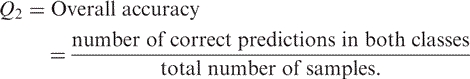
First, we used the overall two-state accuracy (often referred to as _Q_2):
 |
2 |
|---|
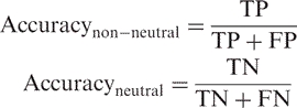
This value alone does not suffice. Therefore, we also compiled the measures listed below [Equations (3) and (4)] and a few others (Table SOM_3, Supplementary Data).
 |
3 |
|---|
 |
4 |
|---|
where TP are the true positives (i.e. correctly predicted non-neutral SNPs) and FP are the false positives (i.e. neutral SNPs predicted to be non-neutral). Similarly, TN are the true negatives (i.e. correctly predicted neutral SNPs) and FN are the false negatives (i.e. non-neutral SNPs predicted to be neutral; Table SOM_4, Supplementary Data). We monitored levels of neutral/non-neutral accuracy and coverage as a function of the reliability index of prediction [Equation (6)]. A trade-off between these two is seen: a higher RI indicates better accuracy (more predictions correspond to observations), but lower coverage (fewer predictions of this type are made). Additionally, higher non-neutral accuracy corresponds to higher neutral coverage and vice versa.
Estimates for standard errors
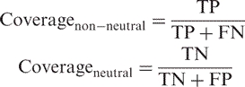
Standard deviation and error for all measurements were estimated in one of two ways: over 10 testing sets (PMD/EC set) or over 100 sets produced by bootstrapping (LacI repressor, lysozyme, HIV-1 protease, melanocortin-4 receptor). Bootstrapping (52) was done by randomly selecting (with replacement) sets of n mutants from the original data set. Thus, bootstrapped sets may have contained repeats of one mutant and no instances of another. We then computed the standard deviation (σ) for each test set (xi) through its difference from the overall performance (〈 x 〉). To compute standard error for PMD/EC data set, σ was divided by the square root of sample size [_n_, Equation (5)]:
 |
5 |
|---|
Reliability index
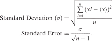
The reliability index (RI) for each prediction was computed by normalizing the difference between the two output units (one for neutral, the other for non-neutral) onto integers between 0 (low reliability) and 9 (high reliability):
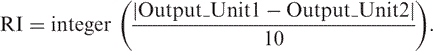 |
6 |
|---|
RESULTS
Feature selection optimized for different classes of solvent accessibility
Which input features predict the functional impact of SNPs best? Two facts complicated the answer to this question. First, our data were inconsistent: annotation varied, e.g. between proteins, between affected tissues, or between experimental laboratories. Second, the data sets were also relatively small in the sense that some 80 K mutants are unlikely to cover the entire variety of all biology (which is essentially what a prediction system implicitly tries to accomplish). To put this point into perspective: for the development of secondary structure prediction methods the 10-fold jump from 100 K to 1 M data points increased performance significantly (55); for the prediction of inter-residue contacts 5 M data points still constitute a small data set (56). Our data set was too small to simply test all possible input features and keep what works best. In order to prevent overfitting, we therefore had to split the data first into subgroups that were likely to be sensitive to different types of changes. For instance, changes of a hydrophobic into a non-hydrophobic amino acid may be non-neutral in the protein core while it may not matter on the surface. We sought good features in three different subsets of buried, intermediate, and exposed residues (Methods section, Table SOM_2, Supplementary Data).
The final network architectures were: 137 input and 45 hidden nodes for buried residues (window length 5; the mutant position plus 2 residues on either side of it), 50 input/35 hidden nodes for intermediate residues (window length 7), and 116 input/20 hidden nodes for exposed residues (window length 3). Increasing window length above 7 consecutive residues did not improve predictions. Shorter windows yielded slightly higher performance for some settings with the clear tendency of ‘shorter toward the protein surface.’ The input feature that had the most descriptive value for all three accessibility classes was the PSIC (3) conservation weight (Methods section).
Except for PSIC, the input features that were best differed by class (Figure SOM_1, Supplementary Data). Best for buried residues were: the simplified PSI-BLAST profile, transition frequencies (likelihood of observing the particular mutation imposed by the SNP), and the predicted values for residue flexibility (from PROFbval). Best for intermediate residues were: relative accessibility scores (PROFacc) and the differences in predicted secondary structure and accessibility caused by the SNP (sequence-only predictions from PROFsec and PROFacc). Best for exposed residues were: the explicit PSI-BLAST profile, accessibility scores (PROFacc), raw secondary structure (PROFsec), and Pfam data.
Best features integrated into SNAP network
Finally, we trained a single network for all classes of solvent accessibility (buried, intermediate, exposed); we included all features that helped in any of the classes. The final SNAP network architecture included the following input features: explicit PSI-BLAST frequency profile, relative solvent accessibility predictions (PROFacc), secondary structure predictions (PROFsec), sequence-only predictions of 1D structure (PROFsec/PROFacc), Pfam information, PSIC scores (Methods section), predicted residue flexibility (PROFbval), and transition frequencies (likelihood of observing the mutation particular mutation imposed by the SNP). With a window length of five consecutive residues, this yielded neural networks with 195 input and 50 hidden units. Note that none of those parameters were optimized on the test sets for which we report performance; instead they all were optimized on the cross-training set (Methods section).
SNAP compared favorably with other tools on the comprehensive PMD/EC data
Evaluated on the PMD/EC data (data sets produced by merging PMD and enzyme data; Methods), SNAP reached a higher level of overall two-state accuracy [78%, Equation (2)] than SIFT (74%) and PolyPhen (75%; Table 1). Given an estimated standard error below two percentage points, this suggested that SNAP outperformed SIFT and PolyPhen. The inclusion of SWISS-PROT annotations and SIFT predictions into the input vector of SNAP (SNAPannotated in Table 1) improved performance even further for both un-annotated proteins (79%; note: only SIFT predictions) and annotated ones (81%).
Table 1.
Performance on PMD/EC set*
| Unk** | Accuracy non-neutral | Coverage non-neutral | Accuracy neutral | Coverage neutral | Overall two-state accuracy | |
|---|---|---|---|---|---|---|
| SIFT | 2374 | 79.8 ± 0.6 | 63.4 ± 1.2 | 70.1 ± 2.7 | 84.3 ± 1.2 | 74.0 ± 1.4 |
| PolyPhen | 1647 | 79.1 ± 0.7 | 66.9 ± 1.4 | 71.8 ± 2.7 | 82.7 ± 1.1 | 74.9 ± 1.3 |
| SNAP | 0 | 76.7 ± 0.7 | 80.2 ± 0.9 | 79.8 ± 2.7 | 76.2 ± 2.2 | 78.2 ± 1.3 |
| SNAPannotated | 0 | 76.3 ± 0.8 | 83.3 ± 1.0 | 82.0 ± 2.4 | 74.7 ± 2.2 | 78.9 ± 1.3 |
Other methods appeared to reach similar levels of accuracy suggesting that the majority of mutants in the data set were classified similarly by all methods. This, however, turned out to be a rushed inference, e.g. SNAPannotated correctly predicted when the one or both of the others (SIFT/PolyPhen) were wrong ∼1.7 times more often than vice versa (SNAPannotated right 10 124 times when SIFT or PolyPhen were wrong; SNAPannotated wrong 6117 times when SIFT or PolyPhen were right.) In other words, for a large subset of the PMD data set (16 241 mutants) for which at least one method was wrong (i.e. mutants with hard-to-establish functional effects), SNAPannotated achieved an overall accuracy of 62.3%, while both PolyPhen (7966 right and 8275 wrong) and SIFT (7566 right and 8675 wrong) attained levels <50% accuracy.
Performance estimates largely confirmed by independent data sets
All our optimizations were performed on PMD/EC data sets (Methods). We carefully avoided over-optimistic estimates by a full rotation through three-way 10-fold cross-validation: training set for optimization of network connections, cross-training set for optimization of all other free parameters (hidden units, type of input, etc.), and the test set for assessing performance. Despite having applied this time-intensive caution, we wanted to test yet another independent data set. Overall, the PMD/EC-based estimates of performance for SNAP were confirmed by the other data sets (Table 2), namely for the E. coli LacI repressor, bacteriophage T4 lysozyme, HIV-1 protease, and human Melanocortin-4 receptor data (Methods). Although these data sets comprehensively sampled the space of possible mutations and carefully evaluated their effects, they covered a minute fraction of the entire sequence space (four proteins; only one from a mammal) and may therefore be less representative than the PMD/EC data. While these additional data were too limited to suggest firm conclusions, they helped to confirm trends. All methods performed slightly less accurately in terms of the average over all these data than over our PMD/EC data. The only overlap between these data sets and the PMD/EC data was in about one quarter of the LacI mutants (they all were contained in the data used for the development/assessment of SIFT and PolyPhen). SNAP still outperformed the competitors on LacI repressor, Lysozyme, and Melanocortin-4 data. The performance was radically different for the viral sequence: PolyPhen produced no predictions for any of its mutants and SNAP performed clearly worse than SIFT. This disparity might originate from the different features used by each method: SIFT bases its predictions only on alignments. In contrast, PolyPhen and SNAP also consider other characteristics (e.g. estimates of secondary structure, functional regions) that may have been misleading for this particular case.
Table 2.
Performance on other data sets*
| Method | LacI repressor | Lysozyme | HIV-1 protease | Melanocortin-4 receptor |
|---|---|---|---|---|
| Standard deviation | 3.3 | 3.7 | 3.2 | 3.5 |
| SIFT | 69.4 | 67.6 | 78.3 | 57.8 |
| PolyPhen | 68.7 | 57.9 | *** | 51.1 |
| SNAP | 70.7 | 70.0 | 68.5 | 71.1 |
| SNAPannotated | 72.7 | 73.2 | 72.3 | 75.5 |
| SNPs3D | ** | ** | ** | 62.2 |
High performance throughout the entire spectrum of accuracy versus coverage
The SNAP predictions were not binary (neutral or non-neutral); instead, they were computed as a difference between the two output units (one for neutral, the other for non-neutral; difference ranged from −100 to 100). ‘Dialing’ through different decision thresholds (which difference yields a prediction of ‘neutral’?) will enable users to decide which of the two flip sides of the same accuracy-coverage coin is more important to them. On the one end of the spectrum, predictions with very high differences are very accurate but will cover very few of the SNPs. On the other end, predictions with very low differences will capture all SNPs but this will be paid for with a significantly reduced accuracy. Thus, dialing through the thresholds generated ROC-like curves for accuracy versus coverage (Figure 1). While the predictions of SIFT are also scaled, the SIFT performance has been optimized for the default cutoff (arrow in Figure 1). PolyPhen predictions do not have numerical values; instead they are sorted into four categories (benign, possibly damaging, probably damaging and unknown). Thus, given our assumption of classifying unknowns into the benign group, only two points exist on PolyPhen's graph: one that sorts all damaging values into the non-neutral class and another that assigns ‘possibly damaging’ SNPs to the benign category. Since ROC-like curves were only available for our methods and only partially for SIFT we didn't compare methods by their ‘area under the curve’ values. However, SNAP clearly outperformed both PolyPhen and SIFT throughout the ROC-like curves (Figure 1). SNAP was only outperformed by SNAPannotated, i.e. the version that also considered SIFT predictions and—when available—SWISS-PROT annotations.
Figure 1.

Performance on PMD/EC data. ROC-like curves giving accuracy versus coverage [Equation (2)] for different prediction methods. SIFT predictions range from 0 to 1; thus the performance of SIFT can be analyzed for the entire accuracy/coverage spectrum, however, SIFT has been evaluated using a default threshold of 0.05. PolyPhen predictions are not scaled; instead, they are sorted by the gravity of the impact (benign, possibly damaging, probably damaging and unknown). Therefore, we could not ‘dial’ through the PolyPhen cutoff to generate a ROC-like curve for PolyPhen. Two points on the graph indicate the difference in performance due to assignment of ‘possibly damaging’ class to non-neutral or neutral categories (default ‘possibly damaging’ = damaging). SNAP and SNAPannotated default thresholds are 0. The defaults for each method are indicated by arrows corresponding in color to the method. The left panel (A) gives the performance for non-neutral SNP mutants; the right panel (B) gives the performance for neutral SNP mutants.
Reliability index measure provides more confidence in predictions
The SNAP's two output units provide for an additional measure of confidence of prediction. Intuitively, it is clear that a smaller difference between the values is indicative of lower confidence in the prediction. This is also the reason why accuracy and coverage of predictions are always at a tradeoff. Higher accuracy predictions are received by sampling more at more reliable cutoffs, thereby reducing the total number of trusted samples. To define this reasoning more precisely we introduced the reliability index measure [RI; range 0–9, Equation (6)]. Higher reliability indices correlated strongly with higher accuracy of prediction. However, the majority of predictions is made in the middle of the index range (e.g. RI = 5, Figure 2).
Figure 2.

Stronger predictions more accurate. Stronger SNAP predictions were more accurate. This allowed the introduction of a reliability index for SNAP predictions [Equation (6)]. This index effectively predicted the accuracy of a prediction and thereby enables users to focus on more reliable predictions. The _x_-axis gives the percentage of residues that were predicted above a given reliability index. The actual values of the reliability index (RI) are shown by numbers in italics above the curve for neutral mutations (green), and below the curve for non-neutral mutations (red). The values for 7 and 8 are not explicitly given to avoid confusion. The _y_-axis shows the cumulative percentage of residues correctly predicted of all those predicted with RI ≥ n [accuracy, Equation (2)]. Curves are shown for SNPs with neutral (green diamonds) and non-neutral (red squares) effects. For instance, ∼38% of both types of residues are predicted at indices ≥5; of all the non-neutral mutations predicted at this threshold, about 90% are predicted correctly, and of all the neutral SNPs about ∼92% are predicted correctly.
Performance better for buried than for exposed residues
The SNAP performed better at correctly predicting non-neutral SNPs in the core of proteins (buried residues) than those at the surface (exposed residues, Figure SOM_2, Supplementary Data). This may be due to better-defined constraints responsible for functional consequences of altering buried residues (e.g. structural constraints). Additionally, it may be due to the fact that there were significantly more non-neutral training samples in the data set localized to the buried regions. Different shape of the accuracy/coverage curves for the neutral and non-neutral samples is the result of different ratios of neutral to non-neutral samples in various accessibility classes (Methods section).
DISCUSSION
Features important to conserve function differ between surface and core SNPs
Although many studies have confirmed the importance of structure for functional integrity, none have analyzed mutants in different classes of solvent accessibility (buried, intermediate, exposed). The observation that the optimal input features differed between these three classes (Figure SOM_1, Supplementary Data) supported the intuition of any structural biologist, namely that different biophysical features govern the type of amino acid substitutions that disrupt function of surface and of core residues. For instance, the entire profile/PSSM was useful to determine the effect of substitutions on the surface, while it sufficed to consider the frequencies of the original and the mutant residues at the SNP position to determine the effects in the core. This differential behavior could partially be explained by that internal residues are more constrained by evolution; therefore, it would suffice to know whether or not the mutated residue ever appears in an alignment of related proteins. Surfaces, on the other hand, tend to be less conserved, i.e. many alternatives may be valid; hence, all of these (full PSSM) must be considered to determine the effect of a substitution.
Another example of the difference is the importance of predicted 1D structure (secondary structure and relative solvent accessibility) features for the prediction of SNP effects on the surface (Figure SOM_1, Supplementary Data). Similar findings have been reported by other studies focusing on the prediction of very different aspects of protein function (40,55,56). These 1D features may be particularly important to determining whether a given position is part of a functional site. Active site involvement of a buried residue, on the other hand, can hypothetically be approximated through assessing its flexibility. Indeed, this would also explain why the predicted flexibility appeared relatively more relevant for buried residues. Fewer and less-descriptive features required by the intermediate residue network may indicate the need for structural or functional characteristics that were not tested and/or for finer gradation of the data in terms of accessibility.
One crucial aspect of the success of SNAP was the way in which we generated additional data for presumed neutral substitutions (anything that is changed between two non-trivially related enzymes both of which have the same experimentally characterized EC number). Interestingly, the performance of SNAP differed substantially between the set of experimentally neutral (less accurate) and presumed neutral substitutions (more accurate). Complete experimental assessments of all possible substitutions are almost impossible. Studies generally evaluate mutations suspected in causing some phenotype. The absence of changes is reported as neutral although it may in fact be non-neutral by some other phenotype. Thus, ‘neutrals’ from PMD may be less reliable than those extracted from enzyme alignments.
Evolutionary information most important, followed by structural information
The types of predicted features of protein structure and function that we used as input contributed to the significant improvements of SNAP. However, the most important single feature, other than the biophysical nature of the mutant and wild type amino acids, was the conservation in a family of related proteins (as measured by the PSIC conservation weight). This finding confirmed results from statistical methods applied by Chasman and Adams (11).
For exposed and buried SNPs another phylogenic feature, namely the detailed PSSM/profile from the PSI-BLAST alignment, was the second most relevant input information. Surprisingly, the information from SWISS-PROT and Pfam annotations did neither clearly improve all predictions, nor all accessibility types (more relevant for surface residues).
If more detailed aspects of structure and function were available for all proteins, these could be input to networks to improve performance. For instance, Yue and Moult (17), have demonstrated that an SVM (Support Vector Machine, i.e. another machine-learning algorithm) can distinguish mutants involved in monogenic disease by considering structural features of the protein affected by the mutation (e.g. breakage of disulfide bond or over-packing).
PolyPhen also uses available structural features of either the query protein or its homologue (>50% pairwise sequence identity to experimental structure required); its structural features include solvent accessibility, secondary structure, phi-psi dihedral angles, ligand binding, inter-chain contacts, functional residue contacts (as annotated in SWISS-PROT), and normalized B-factors. For proteins for which this data is available, PolyPhen slightly out-performed both SNAP and SNAPannotated (Figure 3B, ‘Structure’). However, these cases constituted a very small fraction of all the examples for which we had experimental information about SNP effects (Figure 3A).
Figure 3.

SNAP versus PolyPhen on subsets of PMD/EC data. PolyPhen uses different types of input information. Here, we separately analyzed the relevance of each of these sources. Annotation: residues for which sequence annotations were available (e.g. binding site or transmembrane region), Structure: residues for which experimental structural constraints were available, Alignment: residues for which only alignments (PSIC scores) were available, and Unknown: residues that were not classified by PolyPhen. The bars for All give the performance on the entire data set for orientation. (A) Total number of correct predictions in each class, (B) Accuracy in each group [Equation (2)]. For the experimental annotations in the PMD/EC data set, only alignment information was available for most mutants. SNAP performs slightly better than PolyPhen in the absence of experimental 3D structure and/or annotation, and slightly worse otherwise. Including SWISS-PROT annotations and SIFT predictions into SNAP improved performance for all groups.
The performance of SNAP improved significantly through using available annotations (Figure 3). SWISS-PROT indications of active site, mutagen, transmembrane, binding, and otherwise important regions (Methods) allowed for better identification of possibly non-neutral mutations. For instance, using SNAPannotated to predict the effects of SNPs in Melanocortin-4 corrected 2 of the 13 incorrect SNAP predictions of non-neutral effects (data not shown).
In the absence of annotations for structure and function, the most valuable information is extracted from alignments and family/domain data (Figure 3). A similar finding has been reported previously; namely in the absence of known 3D structure, evolutionary information was most relevant to predict SNP effects (16).
SNAP was more sensitive to severe changes
The distinction of mutants according to the severity of functional effects illustrated the performance of SNAP from a different angle. The difference between the two output nodes of SNAP ranges from −100 to 100; differences ≥1 are considered non-neutral by default. Higher differences correspond to more reliable predictions (Figure 1). SNAP was trained only on experimental data of binary nature, i.e. the supervised output was either labeled as non-neutral or as neutral. Did the network learn implicitly to distinguish between more and less severe effects? We did not have enough data to analyze this question rigorously. We did however have limited data sets (LacI repressor data set containing 4041 mutants) and a limited grading of severity (neutral/slightly damaging/damaging/severe) to explore this question. SNAP clearly performed better on more severe effects (Figure 4, red bars dominate on the right hand side) and clearly ‘more neutral’ (Figure 4, green bars dominate left hand side) changes than those with intermediate effects. This suggested that the difference between the output values did not only reflect the reliability of predictions, but also the severity of the change. Put differently, more severe effects corresponded to stronger SNAP predictions. The reason why SNAP implicitly learned about the severity of effects was likely of statistical nature: the most severe and most neutral mutations were most consistent in the data set.
Figure 4.
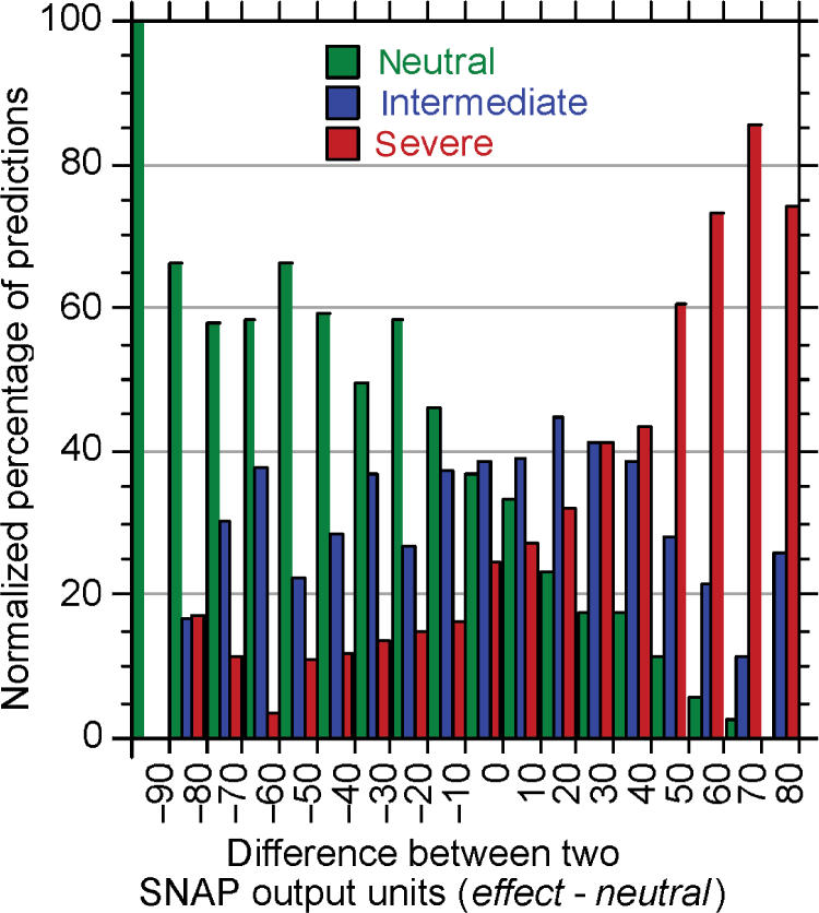
Stronger signals for more severe changes. The reliability index [Equation (6)] of SNAP reflected prediction accuracy (Figure 2). However, we also observed that more severe changes were predicted more reliably, i.e. resulted in a higher difference between the two output units of SNAP. In order to distinguish mutants according to the severity of the change they cause, we used the functional effects observed for the LacI repressor (set from (12), as used in testing SIFT). Samples in the ‘very slightly damaging’ and ‘slightly damaging’ category were combined into a single ‘intermediate’ category. Given are normalized percentages of samples in each category (_y_-axis) for a given range of difference values (_x_-axis). We normalized the predictions in each ‘severity group’ because the samples for ‘intermediate effects’ were significantly under-represented in the experimental data.
The levels of accuracy of prediction attained by SNAP are probably not high enough to make the tool widely useful in genetic counseling applications. However, this correlation of severity of change with the reliability index of prediction makes SNAP highly applicable to prioritization of suspects from disease-association studies for follow-up investigations.
SNAP could predict gain of function as well as loss of function
There is a number of nsSNPs in the PMD data set that are known to introduce ‘gain of function’ for a particular protein. Unfortunately, many mutations entail a gain of one function, but a loss, or retention at same levels, of another. Additionally, modifications that lead to loss of function in one protein may very well correlate with a gain of function in another (e.g. increased structural flexibility may suppress or promote function). Given this reality, we chose not to separate out directions of effects of mutation: for the purposes of SNAP a gain of function is treated as a non-neutral sample. However, to illustrate that SNAP can recognize these mutants consider an example of a few nsSNPs of the metalloendopeptidase thermolysin (EC.3.4.24.). A study (57) of this enzyme, described in PMD, showed that set of 18 nsSNPs of thermolysin increase its activity (‘gain of function’). SNAP correctly identified all of these mutations as non-neutral, with reliability index range 0–5. Although SNAP is already capable of recognizing gain of function changes, it would likely benefit from seeing more of this sort of mutants. However, extensive data of this type is not currently available.
SNAP designed to accommodate the needs of large-scale experimental scans
Two features of SNAP make it particularly useful to researchers who want to scan large experimental data sets. The first is SNAP's particular strength is the correct predictions for the least obvious cases (those for which existing methods disagree). For such mutants SNAP was 13–17% points more accurate than other methods. Furthermore, these mutants are generally also the hardest to pinpoint experimentally since their subtle effects are more likely to contribute to a phenotype rather than fully account for it. In a typical experimental scenario in which experimental observations are likely to have already been subjected to various analysis tools, this improvement is likely to be extremely relevant and significant. For example, for the Melanocortin-4 receptor mutants (Methods and Table 2; C. Vaisse personal communication), SNAP recognized significantly more damaging mutations than other methods. For instance, the Arg18Cys mutation, known to decrease protein basal activity (58), was found to be non-neutral only by SNAP. Similarly, PolyPhen and SIFT also failed to recognize the deleterious Asn97Asp mutant, known to strongly affect ligand binding (59). Overall, SNAP was wrong in only two of the nineteen instances in which at least one of the four methods tested was right; in comparison SIFT was wrong 10/19, PolyPhen 13/19, and SNPs3D 8/19. Had SNAP been available earlier, it would have been a significantly better choice for selecting candidates than any other method. The analysis of the Melanocortin-4 receptor appeared representative in light of a similar analysis for our large data set. The second important novel feature of SNAP is the introduction of a reliability index that correlates with prediction accuracy (Figure 2) and allows filtering out low accuracy predictions. In addition to providing an estimate about the accuracy, the reliability index also reflects the strength of a functional effect (Figure 4). This feature is entirely unique for SNAP.
Will more and better experimental data improve SNAP in the future?
We established that training separate networks on separate classes of solvent accessibility was beneficial, in principle. Unfortunately, the split yielded too small data sets. We expect to need 2–5 times more accurate experimental samples to improve performance. Furthermore, even the available data were not ideal as illustrated by the differences of functional assignments for the 55 mutants from the LacI repressor between the data set used for SNAP and those used for SIFT: 51 of these were considered as non-neutral in training SNAP, while they were classified as neutral by the authors of SIFT. We found that these assignments came from different studies and not from annotation mistakes. Different experimental methods and/or interpretations of results can introduce noise. Moreover, these data tend to be particularly inconsistent across species and across protein families, since a qualitative description of what constitutes an important change often differs across these experimental territories.
In order to somehow accommodate these differences in our evaluation, we annotated SNPs as non-neutral whenever there were different functional annotations. This approach somehow helped our method to cope with alternative annotations, to disregard the direction of change (gain or loss of function), and the severity of a change (mild or severe). It is still clear that noise in the data hampers the development of a better method. Arguably, mutants at the borderline of neutral/non-neutral are most important. For instance, a single mutant associated with a polygenic disorder may not change function globally; instead it may be the conjunction of several mutants that makes the difference. However, we assume that better predictions for the effect of single mutants will be the only means of improving the prediction for complex traits, i.e. polygenic disorders, and that better experimental data will directly translate to better prediction methods applying the same framework that we described.
CONCLUSION
We developed SNAP, a neural-network based tool to be used for the evaluation of functional effects single amino acid substitutions in proteins. SNAP utilizes various biophysical characteristics of the substitution, as well as evolutionary information, some predicted—or when made available observed—structural features, and possibly annotations, to predict whether or not a mutation is likely to alter protein function (in either direction: gain or loss). Although such predictions are already available from other methods, SNAP added important novelty. Amongst the novel aspects was the improved performance throughout the entire spectrum of accuracy/coverage thresholds and the provision of a reliability index that enables users to either zoom into very few very accurate predictions, or to knowingly broadcast less reliable ones. The improved performance translated to many unique and accurate predictions in our data set. We believe that better future experimental data will directly translate to better performance of any prediction method. In the meantime, experimentalists may already speed up their research by using our novel method.
SUPPLEMENTARY DATA
Supplementary Data are available at NAR Online.
[Supplementary Material]
ACKNOWLEDGEMENTS
Thanks to Jinfeng Liu, Andrew Kernytsky, Marco Punta, Avner Schlessinger, and Guy Yachdav (Columbia) for all help; thanks to Chani Weinreb for help with all methods and Kazimierz O. Wrzeszczynski and Dariusz Przybylski (Columbia) for help with the manuscript. Particular thanks to Rudolph L. Leibel (Columbia University) for valuable support, important discussions and the crucial supply of ‘real-life’ data sets. The authors would also like to express gratitude to Christian Vaisse and Cedric Govaerts for the Melanocortin-4 data set. Last, but not least, thanks to all those who deposit their experimental results into public databases and to those who maintain these resources. Y.B. was partially supported by the NLM Medical Informatics Research Training Grant (5-T15-LM007079-15). Funding to pay the Open Access publication charges for this article was provided by the National Library of Medicine (NLM), grant 2-R01-LM007329-05.
Conflict of interest statement. None declared.
REFERENCES
- 1.Kawabata T, Ota M, Nishikawa K. The protein mutant database. Nucleic Acids Res. 1999;27:355–357. doi: 10.1093/nar/27.1.355. [DOI] [PMC free article] [PubMed] [Google Scholar]
- 2.Nishikawa K, Ishino S, Takenaka H, Norioka N, Hirai T, Yao T, Seto Y. Constructing a protein mutant database. Protein Eng. 1994;7:773. doi: 10.1093/protein/7.5.733. [DOI] [PubMed] [Google Scholar]
- 3.Sunyaev SR, Eisenhaber F, Rodchenkov IV, Eisenhaber B, Tumanyan VG, Kuznetsov EN. PSIC: profile extraction from sequence alighnments with position-specific counts of independent observations. Protein Eng. 1999;12:387–394. doi: 10.1093/protein/12.5.387. [DOI] [PubMed] [Google Scholar]
- 4.Chakravarti A. To a future of genetic medicine. Nature. 2001;409:822–823. doi: 10.1038/35057281. [DOI] [PubMed] [Google Scholar]
- 5.The FANTOM Consortium. Carninci P, Kasukawa T, Katayama S, Gough J, Frith MC, Maeda N, Oyama R, Ravasi T, et al. The Transcriptional landscape of the mammalian genome. Science. 2005;309:1559–1563. doi: 10.1126/science.1112014. [DOI] [PubMed] [Google Scholar]
- 6.Liu J, Gough J, Rost B. Distinguishing protein-coding from non-coding RNA through support vector machines. PLoS Genet. 2006;2:e29. doi: 10.1371/journal.pgen.0020029. DOI: 10.1371/journal.pgen.0020029. [DOI] [PMC free article] [PubMed] [Google Scholar]
- 7.Ng PC, Henikoff S. Predicting the effects of amino Acid substitutions on protein function. Annu. Rev. Genomics Hum. Genet. 2006;7:61–80. doi: 10.1146/annurev.genom.7.080505.115630. [DOI] [PubMed] [Google Scholar]
- 8.Wishner BC, Ward KB, Lathman EE, Love WE. Crystal structure of sickle-cell deoxyhemoglobin at 5 A resolution. J. Mol. Biol. 1975;98:179–194. doi: 10.1016/s0022-2836(75)80108-2. [DOI] [PubMed] [Google Scholar]
- 9.Kovacs P, Stumvoll M, Bogardus C, Hanson RL, Baier LJ. A functional Tyr1306Cys variant in LARG is associated with increased insulin action in vivo. Diabetes. 2006;55:1497–1503. doi: 10.2337/db05-1331. [DOI] [PubMed] [Google Scholar]
- 10.Wang Z, Moult J. SNPs, protein structure and disease. Hum. Mutat. 2001;17:263–270. doi: 10.1002/humu.22. [DOI] [PubMed] [Google Scholar]
- 11.Chasman D, Adams RM. Predicting the functional consequences of non-synonymous single nucleotide polymorphisms: structure based assessment of amino acid variation. J. Mol. Biol. 2001;307:683–706. doi: 10.1006/jmbi.2001.4510. [DOI] [PubMed] [Google Scholar]
- 12.Ng PC, Henikoff S. Predicting deleterious amino acid substitutions. Genome Res. 2001;11:863–874. doi: 10.1101/gr.176601. [DOI] [PMC free article] [PubMed] [Google Scholar]
- 13.Ng PC, Henikoff S. Accounting for human polymorphisms predicted to affect protein function. Genome Res. 2002;12:436–446. doi: 10.1101/gr.212802. [DOI] [PMC free article] [PubMed] [Google Scholar]
- 14.Ng PC, Henikoff S. SIFT: predicting amino acid changes that affect protein function. Nucleic Acids Res. 2003;31:3812–3814. doi: 10.1093/nar/gkg509. [DOI] [PMC free article] [PubMed] [Google Scholar]
- 15.Ramensky V, Bork P, Sunyaev SR. Human non-synonymous SNPs: server and survey. Nucleic Acids Res. 2002;30:3894–3900. doi: 10.1093/nar/gkf493. [DOI] [PMC free article] [PubMed] [Google Scholar]
- 16.Saunders CT, Baker D. Evaluation of structural and evolutionary contributions to deleterious mutations prediction. J. Mol. Biol. 2002;322:891–901. doi: 10.1016/s0022-2836(02)00813-6. [DOI] [PubMed] [Google Scholar]
- 17.Yue P, Li Z, Moult J. Loss of protein structure stability as a major causative factor in monogenic disease. J. Mol. Biol. 2005;353:459–463. doi: 10.1016/j.jmb.2005.08.020. [DOI] [PubMed] [Google Scholar]
- 18.Ferrer-Costa C, Orozco M, de la Cruz X. Sequence-based prediction of pathological mutations. Proteins. 2004;57:811–819. doi: 10.1002/prot.20252. [DOI] [PubMed] [Google Scholar]
- 19.Clifford RJ, Edmonson MN, Nguyen C, Scherpbier T, Hu Y, Buetow KH. Bioinformatics tools for single nucleotide polymorphism discovery and analysis. Ann. NY Acad. Sci. 2004;1020:101–109. doi: 10.1196/annals.1310.011. [DOI] [PubMed] [Google Scholar]
- 20.Verzilli CJ, John, Whittaker C, Stallard N, Chasman D. A hierarchical bayesian model for predicting the functional consequences of amino-acid polymorphisms. Appl. Statist. 2005;54:191–206. [Google Scholar]
- 21.Krishnan VG, Westhead DR. A comparative study of machine-learning methods to predict the effects of single nucleotide polymorphisms on protein function. Bioinformatics. 2003;19:2199–2209. doi: 10.1093/bioinformatics/btg297. [DOI] [PubMed] [Google Scholar]
- 22.Capriotti E, Fariselli P, Casadio R. A neural network-based method for predicting protein stability changes upon single point mutation. Bioinformatics. 2004;1:1–6. doi: 10.1093/bioinformatics/bth928. [DOI] [PubMed] [Google Scholar]
- 23.Bao L, Cui Y. Prediction of the phenotypic effects of non-synonymous single nucleotide polymorphisms using structural and evolutionary information. Bioinformatics. 2005;21:2185–2190. doi: 10.1093/bioinformatics/bti365. [DOI] [PubMed] [Google Scholar]
- 24.Cohen JC, Kiss RS, Pertsemlidis A, Marcel YL, McPherson R, Hobbs HH. Multiple rare alleles contribute to low plasma levels of HDL cholesterol. Science. 2004;305:869–872. doi: 10.1126/science.1099870. [DOI] [PubMed] [Google Scholar]
- 25.Letourneau IJ, Deeley RG, Cole SP. Functional characterization of non-synonymous single nucleotide polymorphisms in the gene encoding human multidrug resistance protein 1 (MRP1/ABCC1) Pharmacogenet. Genomics. 2005;15:647–657. doi: 10.1097/01.fpc.0000173484.51807.48. [DOI] [PubMed] [Google Scholar]
- 26.Freimuth RR, Xiao M, Marsh S, Minton M, Addleman N, Van Booven DJ, McLeod HL, Kwok PY. Polymorphism discovery in 51 chemotherapy pathway genes. Hum. Mol. Genet. 2005;14:3595–3603. doi: 10.1093/hmg/ddi387. [DOI] [PubMed] [Google Scholar]
- 27.Sunyaev SR, Ramensky V, Koch I, Lathe WI, Kondrashov AS, Bork P. Prediction of deleterious human alleles. Hum. Mol. Genet. 2001;10:591–597. doi: 10.1093/hmg/10.6.591. [DOI] [PubMed] [Google Scholar]
- 28.Bairoch A, Apweiler R. The SWISS-PROT protein sequence database and its supplement TrEMBL in 2000. Nucleic Acids Res. 2000;28:45–48. doi: 10.1093/nar/28.1.45. [DOI] [PMC free article] [PubMed] [Google Scholar]
- 29.Altschul SF, Madden TL, Schäffer AA, Zhang J, Zhang Z, Miller W, Lipman DJ. Gapped Blast and PSI-Blast: a new generation of protein database search programs. Nucleic Acids Res. 1997;25:3389–3402. doi: 10.1093/nar/25.17.3389. [DOI] [PMC free article] [PubMed] [Google Scholar]
- 30.Sander C, Schneider R. Database of homology-derived structures and the structural meaning of sequence alignment. Proteins. 1991;9:56–68. doi: 10.1002/prot.340090107. [DOI] [PubMed] [Google Scholar]
- 31.Rost B. Twilight zone of protein sequence alignments. Protein Eng. 1999;12:85–94. doi: 10.1093/protein/12.2.85. [DOI] [PubMed] [Google Scholar]
- 32.Markiewicz P, Kleina LG, Cruz C, Ehret S, Miller JH. Genetic studies of the lac repressor. XIV. Analysis of 4000 altered Escherichia coli lac repressors reveals essential and non-essential residues, as well as ‘spacers’ which do not require a specific sequence. J. Mol. Biol. 1994;240:421–433. doi: 10.1006/jmbi.1994.1458. [DOI] [PubMed] [Google Scholar]
- 33.Rennel D, Bouvier SE, Hardy LW, Poteete AR. Systematic mutations of bacteriophage T4 lysozyme. J. Mol. Biol. 1991;222:67–88. doi: 10.1016/0022-2836(91)90738-r. [DOI] [PubMed] [Google Scholar]
- 34.Loeb DD, Swanstrom R, Everitt L, Manchester M, Stamper SE, Hutchison CA. Complete mutagenesis of the HIV-1 protease. Nature. 1989;340:397–400. doi: 10.1038/340397a0. [DOI] [PubMed] [Google Scholar]
- 35.Rost B. In: The Proteomics Protocols Handbook. Walker JE, editor. Totowa, NJ: Humana; 2005. pp. 875–901. [Google Scholar]
- 36.Rost B. PHD: predicting one-dimensional protein structure by profile-based neural networks. Methods Enzymol. 1996;266:525–539. doi: 10.1016/s0076-6879(96)66033-9. [DOI] [PubMed] [Google Scholar]
- 37.Rost B, Sander C. Prediction of protein secondary structure at better than 70% accuracy. J. Mol. Biol. 1993;232:584–599. doi: 10.1006/jmbi.1993.1413. [DOI] [PubMed] [Google Scholar]
- 38.Joachims T. In: Advances in Kernel Methods - Support Vector Learning. Schölkopf B, Burges C, Smola A, editors. Cambridge, MA: MIT-Press; 1999. [Google Scholar]
- 39.Ofran Y, Rost B. Predicted protein-protein interaction sites from local sequence information. FEBS Lett. 2003;544:236–239. doi: 10.1016/s0014-5793(03)00456-3. [DOI] [PubMed] [Google Scholar]
- 40.Nair R, Rost B. Mimicking cellular sorting improves prediction of subcellular localization. J. Mol. Biol. 2005;348:85–100. doi: 10.1016/j.jmb.2005.02.025. [DOI] [PubMed] [Google Scholar]
- 41.Wu CH, Apweiler R, Bairoch A, Natale DA, Barker WC, Boeckmann B, Ferro S, Gasteiger E, Huang H, et al. The Universal Protein Resource (UniProt): an expanding universe of protein information. Nucleic Acids Res. 2006;34:D187–D191. doi: 10.1093/nar/gkj161. [DOI] [PMC free article] [PubMed] [Google Scholar]
- 42.Apweiler R, Bairoch A, Wu CH, Barker WC, Boeckmann B, Ferro S, Gasteiger E, Huang H, Lopez R, et al. UniProt: the universal protein knowledgebase. Nucleic Acids Res. 2004;32:D115–D119. doi: 10.1093/nar/gkh131. [DOI] [PMC free article] [PubMed] [Google Scholar]
- 43.Berman HM, Westbrook J, Feng Z, Gilliland G, Bhat TN, Weissig H, Shindyalov IN, Bourne PE. The protein data bank. Nucleic Acids Res. 2000;28:235–242. doi: 10.1093/nar/28.1.235. [DOI] [PMC free article] [PubMed] [Google Scholar]
- 44.Bairoch A, Apweiler R, Wu CH, Barker WC, Boeckmann B, Ferro S, Gasteiger E, Huang H, Lopez R, et al. The Universal Protein Resource (UniProt) Nucleic Acids Res. 2005;33:D154–D159. doi: 10.1093/nar/gki070. [DOI] [PMC free article] [PubMed] [Google Scholar]
- 45.Thompson JD, Higgins DG, Gibson TJ. CLUSTAL W: improving the sensitivity of progressive multiple sequence alignment through sequence weighting, position-specific gap penalties and weight matrix choice. Nucleic Acids Res. 1994;22:4673–4680. doi: 10.1093/nar/22.22.4673. [DOI] [PMC free article] [PubMed] [Google Scholar]
- 46.Rost B, Sander C. Conservation and prediction of solvent accessibility in protein families. Proteins Struct. Funct. Genet. 1994;20:216–226. doi: 10.1002/prot.340200303. [DOI] [PubMed] [Google Scholar]
- 47.Rost B. How to use protein 1D structure predicted by PROFphd. In: Walker JE, editor. The Proteomics Protocols Handbook. Totowa NJ: Humana; 2005. pp. 875–901. [Google Scholar]
- 48.Schlessinger A, Yachdav G, Rost B. PROFbval: predict flexible and rigid residues in proteins. Bioinformatics. 2006;22:891–893. doi: 10.1093/bioinformatics/btl032. [DOI] [PubMed] [Google Scholar]
- 49.Bateman A, Lachlan C, Durbin R, Finn RD, Hollich V, Griffiths-Jones S, Khanna A, Marshall M, et al. The Pfam Protein Families Database. Nucleic Acids Res. 2004;32:D138–D141. doi: 10.1093/nar/gkh121. [DOI] [PMC free article] [PubMed] [Google Scholar]
- 50.Ng PC, Henikoff JG, Henikoff S. PHAT: a transmembrane-specific substitution matrix. Predicted hydrophobic and transmembrane. Bioinformatics. 2000;16:760–766. doi: 10.1093/bioinformatics/16.9.760. [DOI] [PubMed] [Google Scholar]
- 51.Fu L. Neural Networks in Computer Intelligence. 1st. New York, NY, USA: McGraw-Hill Inc.; 1994. [Google Scholar]
- 52.Efron B, Halloran E, Holmes S. Bootstrap confidence levels for phylogenetic trees. Proc. Natl Acad. Sci. USA. 1996;93:13429–13434. doi: 10.1073/pnas.93.23.13429. [DOI] [PMC free article] [PubMed] [Google Scholar]
- 53.Yeo GS, Lank EJ, Farooqi IS, Keogh J, Challis BG, O’Rahilly S. Mutations in the human melanocortin-4 receptor gene associated with severe familial obesity disrupts receptor function through multiple molecular mechanisms. Hum. Mol. Genet. 2003;12:561–574. doi: 10.1093/hmg/ddg057. [DOI] [PubMed] [Google Scholar]
- 54.Ofran Y, Rost B. ISIS: interaction sites identified from sequence. Bioinformatics. 2007;23:e13–6. doi: 10.1093/bioinformatics/btl303. [DOI] [PubMed] [Google Scholar]
- 55.Rost B. Review: protein secondary structure prediction continues to rise. J. Struct Biol. 2001;134:204–218. doi: 10.1006/jsbi.2001.4336. [DOI] [PubMed] [Google Scholar]
- 56.Punta M, Rost B. PROFcon: novel prediction of long-range contacts. Bioinformatics. 2005;21:2960–2968. doi: 10.1093/bioinformatics/bti454. [DOI] [PubMed] [Google Scholar]
- 57.Schlessinger A, Rost B. Protein flexibility and rigidity predicted from sequence. Proteins Struct. Funct. Bioinform. 2005;61:115–126. doi: 10.1002/prot.20587. [DOI] [PubMed] [Google Scholar]
- 58.Kidokoro S, Miki Y, Endo K, Wada A, Nagao H, Miyake T, Aoyama A, Yoneya T, Kai K, et al. Remarkable activity enhancement of thermolysin mutants. FEBS Lett. 1995;367:73–76. doi: 10.1016/0014-5793(95)00537-j. [DOI] [PubMed] [Google Scholar]
- 59.Govaerts C, Srinivasan S, Shapiro A, Zhang S, Picard F, Clement K, Lubrano-Berthelier C, Vaisse C. Obesity-associated mutations in the melanocortin 4 receptor provide novel insights into its function. Peptides. 2005;26:1909–1919. doi: 10.1016/j.peptides.2004.11.042. [DOI] [PubMed] [Google Scholar]
Associated Data
This section collects any data citations, data availability statements, or supplementary materials included in this article.
Supplementary Materials
[Supplementary Material]