Efficient Control of Population Structure in Model Organism Association Mapping (original) (raw)
Abstract
Genomewide association mapping in model organisms such as inbred mouse strains is a promising approach for the identification of risk factors related to human diseases. However, genetic association studies in inbred model organisms are confronted by the problem of complex population structure among strains. This induces inflated false positive rates, which cannot be corrected using standard approaches applied in human association studies such as genomic control or structured association. Recent studies demonstrated that mixed models successfully correct for the genetic relatedness in association mapping in maize and Arabidopsis panel data sets. However, the currently available mixed-model methods suffer from computational inefficiency. In this article, we propose a new method, efficient mixed-model association (EMMA), which corrects for population structure and genetic relatedness in model organism association mapping. Our method takes advantage of the specific nature of the optimization problem in applying mixed models for association mapping, which allows us to substantially increase the computational speed and reliability of the results. We applied EMMA to in silico whole-genome association mapping of inbred mouse strains involving hundreds of thousands of SNPs, in addition to Arabidopsis and maize data sets. We also performed extensive simulation studies to estimate the statistical power of EMMA under various SNP effects, varying degrees of population structure, and differing numbers of multiple measurements per strain. Despite the limited power of inbred mouse association mapping due to the limited number of available inbred strains, we are able to identify significantly associated SNPs, which fall into known QTL or genes identified through previous studies while avoiding an inflation of false positives. An R package implementation and webserver of our EMMA method are publicly available.
WITH the recent development of high-throughput genotyping technologies, genetic variation in many model organisms such as mice, Arabidopsis, and maize is being discovered on a genomewide scale (Jander et al. 2002; Pletcher et al. 2004; Flint-Garcia et al. 2005; Frazer et al. 2007). Genomewide association mapping in model organisms has great potential to identify risk factors for complex traits related to human diseases. Despite the disadvantage that direct inferences from model organisms are not always applicable to human traits, model organism association mapping is potentially more powerful than human association mapping because it is possible to reduce the effect of environmental factors by replicating phenotype measurements in genetically identical organisms (Belknap 1998). In addition, it is often easier and more cost effective to verify associated signals in model organisms than in human subjects. Moreover, many ongoing genotyping and phenotyping projects in model organisms such as the Mouse Phenome Database (MPD) (http://www.jax.org/phenome), the Mouse HapMap project (http://www.broad.mit.edu/personal/claire/MouseHapMap), and the Perlegen/NIEHS resequencing project (http://mouse.perlegen.com) (Frazer et al. 2007) provide publicly available resources to perform in silico mapping of complex traits in model organisms (Peter et al. 2007).
However, genetic association studies in inbred model organisms are confronted by the problem of inflated false positive rates due to population structure and genetic relatedness among inbred strains caused by the complex genealogical history of most model organism strains. Conventional statistical tests of independence between a genetic marker and a phenotype are prone to spurious associations because the marker and the phenotype are likely to be correlated due to population structure that violates the independence assumption under the null hypothesis. Recent association- or linkage-mapping studies in model organisms attempt to avoid inflated false positive rates by designing the studies using recombinant inbred lines generated from a small number of parental strains (Bystrykh et al. 2005; Zou et al. 2005). However, these studies are limited by the variation present in the parental strains and have long regions between recombinations due to relatively few generations between the recombinant inbred strains and the parental strains. Traditional QTL mapping using F2 or backcross suffers from the same problem in fine-resolution mapping in addition to expensive genotyping cost (Belknap 1998; Flint et al. 2005).
An alternative approach to reduce the inflation of false positives is to apply a statistical test that corrects for the bias due to population structure or genetic relatedness. The most widely used methods to reduce such bias in human association mapping are genomic control (Devlin and Roeder 1999), structured association (Pritchard et al. 2000), and principal component analysis (Patterson et al. 2006; Price et al. 2006). However, these methods are inadequate in the case of model organism association mapping. Genomic control suffers from weak power when the effect of population structure is large as in model organisms (Price et al. 2006; Yu et al. 2006). Structured association or principal component analysis, which assumes a small number of ancestral populations and admixture, only partially captures the multiple levels of population structure and genetic relatedness in model organisms (Aranzana et al. 2005; Yu et al. 2006; Zhao et al. 2007). Recently, it has been suggested that linear mixed models can effectively correct for population structure in the association mapping of quantitative traits (Yu et al. 2006). Linear mixed models incorporate pairwise genetic relatedness between every pair of individuals in the statistical model directly, reflecting that the phenotypes of two genetically similar individuals are more likely to be correlated than genetically dissimilar individuals. Applications of mixed models to association mapping in maize, Arabidopsis, and potato panels demonstrate that mixed models obtain fewer false positives and higher power than previous methods including genomic control, structured association, and principal component analysis (Yu et al. 2006; Malosetti et al. 2007; Zhao et al. 2007).
Although mixed models can effectively capture statistical confounding due to population structure, the currently available implementations have several limitations in the context of model organism association mapping. First, the variance components numerically estimated by various hill-climbing approaches such as the Nelder–Mead simplex algorithm (Nelder and Mead 1965; Graser et al. 1987; Meyer 1989), the EM algorithm (Smith 1990), and the Newton–Raphson algorithm (Lindstrom and Bates 1988; Gilmour et al. 1995; Johnson and Thompson 1995) provide only a locally optimal solution, which may cause the statistical inferences based on these estimates to be inaccurate. Second, the computational cost of the numerical optimization procedure is substantial, requiring a large number of computationally expensive matrix operations at each iteration. Computational considerations are important when large data sets are to be tested. For example, the association mapping with maize panels consisting of hundreds of SNPs over hundreds of strains takes hours for a single run with currently available implementations such as TASSEL (Yu et al. 2006) or SAS (Sas Institute 2004). A microarray data set tested for genomewide association mapping between thousands of transcripts and tens of thousands of markers would take several years of CPU time. Third, when inferring the genetic variance component referred to as the kinship matrix, the importance of a mathematically correct form of kinship matrix estimation is often overlooked. For example, Yu et al. (2006) proposed to infer a kinship matrix using SPAGeDi software, setting negative kinship coefficients to zero. Such a kinship matrix may not be positive semidefinite and thus not be a valid form of variance component. Using a nonpositive semidefinite kinship matrix generates ill-defined likelihood for a subset of parameter space in the estimation of the variance component.
In this article, we propose a new method, efficient mixed-model association (EMMA), which corrects for population structure and genetic relatedness in model organism association mapping. Our method takes advantage of the specific nature of the optimization problem in applying mixed models for association mapping, which allows us to substantially increase computational speed by orders of magnitude and improve the reliability of results by achieving near global optimization. Our method improves the efficiency of the mixed-model method by enabling us to perform statistical tests with single-dimensional optimization. Our method's efficiency is further increased by avoiding redundant computationally expensive matrix operation at each iteration in the computation of likelihood function by leveraging spectral decomposition, reducing the computational cost of each iteration from cubic to linear complexity. Due to a substantially decreased computational cost of each iteration, it is possible to converge the global optimum of the likelihood in variance-component estimation with high confidence by combining grid search and the Newton–Raphson algorithm even though the likelihood function may not be convex. Our method is related to a similar technique developed in a different context of simulating the null distribution of variance-component test statistics (Crainiceanu and Ruppert 2004).
We show that a simple genetic similarity matrix can serve as a kinship matrix accounting for genetic relatedness as effectively as previously suggested methods while guaranteeing positive semidefiniteness. Our results are consistent with other studies (Zhao et al. 2007), which suggests that these simpler kinship matrices reduce the false positive rate as effectively as or more effectively than the kinship matrices generated by previous methods (Yu et al. 2006). We propose an additional method called phylogenetic control based on the assumption that a phylogenetic tree is a good approximation of the genealogical history of an inbred model organism. In such cases, the phylogenetic tree may be used as a confounding factor, correcting for the complex genetic relations between strains. We show that phylogenetic control can be formulated as a linear mixed model and present an algorithm for inferring the phylogenetic kinship matrix. We show that the phylogenetic kinship matrix is always positive semidefinite and its optimal variance components are unique regardless of the choice of root.
One of the important questions in the design of model organism association-mapping studies is estimating the statistical power for any specific set of inbred strains. We performed a simulation study of the power of our EMMA method to identify causal SNPs both on a genomewide scale and within a smaller region such as a QTL interval. Our results show that with a limited number of genetically diverse strains, such as the currently available panel of inbred mice, it is possible to identify causal loci with a genomewide significance only if the locus explains a large portion of phenotypic variance. However, with more strains, the power of these association studies increases dramatically. Our analysis of statistical power in model organism association mapping demonstrates the dramatic increase in power using multiple measurements of phenotypes from multiple animals for each strain. Study designs that do not replicate phenotype measurements and analysis methods that do not take individual measurements into account suffer a significant decrease in statistical power.
We applied our EMMA method to association mappings of various inbred model organisms. First, we verified that EMMA gives almost identical results to other widely used implementations using the maize panel data sets (Yu et al. 2006). In terms of computational time, EMMA is shown to be orders of magnitude faster than the previous methods while performing near global optimization. Second, we performed a genomewide association mapping of Arabidopsis flowering-time phenotypes. Our results are consistent with the recently published results (Zhao et al. 2007), reducing most of the inflated false positives. Finally, we used our EMMA method to perform a whole-genome association-mapping study of inbred mouse strains. We analyzed nearly 140,000 mouse HapMap SNPs over 48 strains and three quantitative phenotypes, liver weight, body weight, and saccharin preference, with QTL identified by previous studies. We identified significant associations for the three phenotypes while our results show a significant reduction in the inflation of false positives. Interestingly, many of the significantly associated SNPs fall into the known QTL, suggesting the results are likely to be true associations.
An R package implementation of EMMA and the webserver containing the mouse association results are publicly available online at http://mouse.cs.ucla.edu/emma.
MATERIALS AND METHODS
Genotypes and phenotypes:
Genotypes, phenotypes, SPAGeDi-based kinship matrix, and the STRUCTURE outputs from 277 maize strains across 553 SNPs as described in Yu et al. (2006) were downloaded from the Buckler lab web site (http://www.maizegenetics.net). The Arabidopsis genotypes and phenotypes and the output from STRUCTURE were obtained from the published data sets (Aranzana et al. 2005; Nordborg et al. 2005). The 13,416 nonsingleton Arabidopsis SNPs with no more than 10% of genotype calls missing were tested for association after imputing the missing alleles using HAP (Halperin and Eskin 2004). The flowering-time phenotypes over 95 strains were log transformed to fit to a normal distribution.
For inbred mouse association mapping, the Broad mouse HapMap SNP sets were obtained from the mouse HapMap web site. The 106,040 SNPs that have no more than 10% of genotype calls missing were tested after imputing the missing alleles. The initial body weight (MPD10305) and liver weight phenotypes (MPD2907) were downloaded from Jackson Laboratory MPD (Jackson Laboratory 2004). They consist of 374 and 308 phenotype measurements over 38 and 34 strains, respectively. The saccharin preference phenotypes consist of 280 phenotype measurements in 24 strains (Reed et al. 2004).
EMMA:
Suppose that n measurements of a phenotype are collected across t inbred strains. A linear mixed model in model organism association mapping is typically expressed as
 |
(1) |
|---|
where y is an n × 1 vector of observed phenotypes, and X is an n × q matrix of fixed effects including mean, SNPs, and other confounding variables.  is a q × 1 vector representing coefficients of the fixed effects. Z is an n × t incidence matrix mapping each observed phenotype to one of t inbred strains. u is the random effect of the mixed model with Var(u) =
  where K is the t × t kinship matrix inferred from genotypes as described in the following section, and e is an n × n matrix of residual effect such that Var(e) =
  The overall phenotypic variance–covariance matrix can be represented as
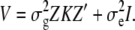
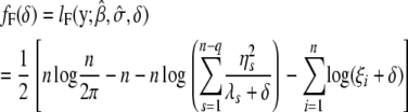
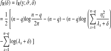
Instead of solving mixed-model equations by obtaining the best linear unbiased prediction (BLUP) of random effects u via Henderson's iterative procedure (Henderson 1984; Arbelbide et al. 2006), we directly estimate the variance components σg and σe, maximizing the full likelihood or restricted likelihood that is defined as full likelihood with the fixed effects integrated out (Dempster et al. 1981). The restricted likelihood avoids a downward bias of maximum-likelihood estimates of variance components by taking into account the loss in degrees of freedom associated with fixed effects. Under the null hypothesis, the full log-likelihood and restricted log-likelihood function can be formulated as
 |
(2) |
|---|
 |
(3) |
|---|
(Welham and Thompson 1997), where σ = σg and H = σ−1_V_ = ZKZ_′ + δ_I is a function of δ, defined as δ = 
The full-likelihood function is maximized when β is 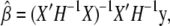 and the optimal variance component is
  for full likelihood and
 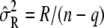 for restricted likelihood, where
 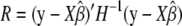 is a function of δ as well.
Using spectral decomposition, it is possible to find ξ_i_ and λ_s_ such that
 |
(4) |
|---|
 |
(5) |
|---|
where S = I − X(X_′_X)−1_X_′, _U_F is n × n, and _U_R is an n × (n − q) eigenvector matrix corresponding to the nonzero eigenvalues. _W_R is an n × q eigenvector matrix corresponding to zero eigenvalues. As shown in the appendix, our decomposition satisfies the properties of the decomposition suggested by previous studies (Patterson and Thompson 1971). It should be noted that _U_F and _U_R are independent of δ. Let  y = [η1, η2, ⋯, η_n_−_q_]′; then finding maximum-likelihood (ML) or restricted maximum-likelihood (REML) estimates is equivalent to optimizing the following functions with respect to δ:
 |
(6) |
|---|
 |
(7) |
|---|
(see the appendix for the mathematical details). The derivatives of these functions follow that
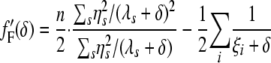 |
(8) |
|---|
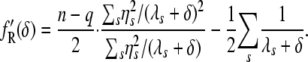 |
(9) |
|---|
It should be noted that the likelihood functions are continuous for all δ > 0 if and only if all the eigenvalues λ_s_ are nonnegative. Otherwise, such as in the case of the nonpositive semidefinite kinship matrix, the likelihood would be ill defined for a certain range of δ.
The suggested procedure in computing likelihood and its derivatives involves only a linear time vector operation at each iteration once the spectral decomposition is computed. The time complexity of the method is O(_n_3 + rn), where r is the number of iterations required. The time complexity of standard EM or Newton–Raphson algorithms is O(_rn_3), and the actual ratio of the running time is much bigger than r because the existing methods typically require a large number of matrix multiplications and inverses at each iteration while EMMA computes spectral decomposition only once. Since the computational cost of each iteration has decreased dramatically, instead of obtaining a locally optimal solution during the numerical optimization, it is now computationally feasible to perform a grid search combining with the Newton–Raphson algorithm in the single-dimensional parameter space consisting of δ, which is the ratio of the environmental random effect to the genetic background effect, to optimize the likelihood globally with high confidence.
Furthermore, when a large number of multiple measurements are phenotyped per strain, i.e.,  , the execution time can be further reduced using the fact that the nonnegative eigenvalues of _ZKZ_′ and SZKZ_′_S are the same as those of KZ_′_Z and KZ_′_SZ, respectively. Combining this fact with a simple modification of the Gram–Schmidt process greatly reduces the execution time of eigenvalue decomposition, reducing the time complexity into O(n_2_t + rn). When multiple phenotypes are tested such as in expression quantitative trait loci (eQTL) mapping, the spectral decomposition can be reused, and only a square-time matrix–vector multiplication is required for each phenotype. Thus, the time complexity with m different phenotypes is O(n_2_t + n_2_m + rmn), which is much more efficient than O(rn_3_m) achieved by previous approaches.
In the application of our EMMA method to the various data sets presented in this article, the δ's ranged from 10−5 (almost pure population structure effect) to 105 (almost pure environmental or residual effect) and are divided evenly into 100 regions in logarithm scale to compute the derivatives of likelihood functions. The global ML or REML is searched for by applying the Newton–Raphson algorithm to all the intervals where the signs of derivatives change and taking the optimal δ among all of the stationary points and endpoints. Since the derivatives of both the full- and the restricted-likelihood function are continuous with nonnegative eigenvalues, such an optimization technique has guaranteed convergence properties as long as the kinship matrix is positive semidefinite. In the following two sections, we describe different methods to infer a kinship matrix K, based on either a genetic similarity matrix or a phylogenetic tree.
Similarity-based kinship matrix:
A number of methods for inferring a kinship matrix from a large number of molecular markers have been suggested, including a simple identical-by-state (IBS) allele-sharing matrix, an allele-frequency weighted IBS matrix (Lynch and Ritland 1999), a maximum-likelihood kinship matrix (Thomas and Hill 2000), and a Monte Carlo simulation-based matrix (Wang 2002). Comparisons of different kinship matrices for explaining genetic differentiation among populations show similar results with small quantitative differences (Nievergelt et al. 2007). Recent studies on the association mapping of Arabidopsis thaliana in a structured population show that a simple IBS allele-sharing matrix effectively corrects for confounding from population structure, even better than more sophisticated methods (Zhao et al. 2007). Although recently suggested estimators of pairwise relatedness have some desirable statistical properties over a simple IBS allele-sharing matrix (Casteele et al. 2001), they are not guaranteed to be positive semidefinite.
Here we show that a simple IBS allele-sharing matrix based on the assumption of each SNP or haplotype inducing the same level of small random changes on the phenotype guarantees positive semidefiniteness and convergence if missing alleles are handled appropriately.
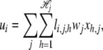
Let li,j,h ∈ {0, 1} be a binary variable that has a value of 1 only when the genotype (or haplotype) allele at _j_th locus in the _i_th strain is  , where
  is the total number of alleles at the _j_th locus. Let xh,j be random variables independently sampled from N(0, σ2); then the genetic background effect ui of strain i can be modeled as an accumulation of small random effects as follows, assuming that xh,j denote the random genetic effect caused by allele h at the _j_th locus,
 |
(10) |
|---|
where wj is the weight of each SNP's contribution to the genetic background effect. If each SNP is assumed to have the same level of random effect, wj = 1 can be assumed. Alternatively, wj can be a function of allele frequency or a function depending on the genomic region of the SNP. Let  and let Lh be the matrix whose element at (i, j) is li,j,h; then the overall genetic background effect u is expressed in the form
 |
(11) |
|---|
where W is a diagonal square matrix with wi at the _i_th diagonal element. Assuming that each xh,j follows a normal distribution with zero mean and variance of σ2 independently, the variance–covariance matrix of u becomes  Since its (_i_0, _i_1)th element
 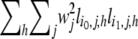 represents the number of shared IBS alleles between the _i_0th and _i_1th strains directly if wj = 1, Var(u) is equivalent to a weighted IBS allele sharing a kinship matrix with the scaling factor σ2. It is obvious from Equation 11 that the kinship matrix is positive semidefinite. When missing genotypes exist, we estimate li,j,h to be the square root of the probability of the SNP or haplotype allele at the _j_th locus having the allele h. This is so the random effect for each allele is assigned probabilistically. We generated genotype similarity of maize, Arabidopsis, and mouse data sets using uniform weight. When a haplotype similarity matrix is used, the haplotype window size resulting in the largest ML estimates is selected as the optimal window size. In the Arabidopsis and mouse association-mapping results of this article, the optimal haplotype window size is set to five in both cases.
Phylogenetic control:
Evolutionary biologists have modeled interspecific phenotype distribution using various phylogenetic comparative methods (PCMs) (Martins and Hansen 1997). The correlation structure between phenotypes can be effectively captured with phylogenetic trees, and PCMs have been applied to evolutionary analysis of quantitative traits such as gene expression (Gu 2004; Oakley et al. 2005) or, very recently, to the association mapping of dichotomous phenotypes (Bhattacharya et al. 2007; Carlson et al. 2007). Felsentein's independent contrast (FIC) method (Felsenstein 1985) models the correlation between phenotypes under the assumption of Brownian motion of phenotypic change along the phylogeny. Since random phenotypic changes occur within a species as well, in cases where the phylogenetic tree is a good approximation of genealogical history, it is reasonable to apply PCMs such as the FIC method in modeling the phenotypic variation in model organisms.
We followed Felsenstein's assumption of Brownian phenotypic changes along the phylogeny. Although multiple fluctuating selection may lead to a Brownian motion model (Felsenstein 1981), here we assume a neutral model where phenotypic changes are explained by accumulated random pleiotropic effects by the genetic background to mathematically model Brownian phenotypic changes. Let T be a phylogenetic tree with t leafs and m edges, and let z ∈ Rm be random variables independently sampled from  At each branch i whose length is bi, we represent the amount of random phenotypic changes along the branch as
  Let Ψ_i_ denote the set of branches connecting to a leaf node i from the root. Then the accumulated phenotypic changes are equivalent to
  If
If  is the ancestral mean at an arbitrarily chosen root node, then the phenotype values at the leaf nodes are expressed in the form
 |
(12) |
|---|
where E is a t × m matrix whose (i, j)th element is  if branch j exists in the path from the root to the leaf node i and zero otherwise. The kinship matrix of random effect u = Ez is K = _EE_′ and is proportional to its covariance. If the root of the phylogenetic tree changes, E is changed into E + 1tcT, with 1t a vector of ones and another vector c. However, the restricted likelihood does not change because SZ1t = 0 always holds.
In our results, we adjusted the genetic distance matrix using the F84 model (Kishino and Hasegawa 1989; Felsenstein and Churchill 1996) from the genomewide genotypes and inferred the phylogenetic tree with the Fitch–Margoliash and least-squares distance method (Fitch and Margoliash 1967).
Statistical tests and multiple hypothesis testing:
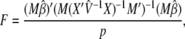
Once the ML or REML variance component  is estimated, a general _F_-statistic testing the null hypothesis _M_β = 0 for an arbitrary full-rank p × q matrix M can be constructed as suggested in Kennedy et al. (1992) and Yu et al. (2006),
 |
(13) |
|---|
with p numerator degrees of freedom and n − q denominator degrees of freedom. The Satterthwaite degrees of freedom may also be computed, avoiding computationally intensive matrix operations.
The likelihood-ratio test can also be performed on the basis of the estimated ML variance components under different fixed effects. The statistic asymptotically follows a  distribution unless the estimated variation component meets the boundary of parameter space.
When a large number of correlated SNPs are tested, Bonferroni correction may lead to too conservative type I error control. Alternatively, permutation tests or other multiple hypothesis-testing procedures can be used (Piepho 2001; Storey and Tibshirani 2003). If permutations of simulation-based approaches are applied, the computational cost is much larger but can be reduced by reusing the spectral decomposition in the same way described in the context of multiple phenotypes. For each permuted y, only  y = [η1, η2, ⋯, η_n_−_q_] has to be computed again to compute the full or the restricted likelihood in linear time at each iteration. Thus, the computational cost for a cubic-time spectral decomposition at each permutation can be substituted by a square-time matrix–vector multiplication, reducing the overall time complexity from O(n_2_t + rn) to O(_n_2 + rn).
The variance-component estimation is performed on the basis of REML for the _F_-test, and ML estimations are used for the likelihood-ratio test and the computation of the Bayesian information criterion (BIC). The _P_-values are computed from the asymptotic null distribution.
Simulation studies:
We performed two simulation studies for analyzing the statistical power of EMMA. The first simulation is similar to those from other mixed-model studies (Yu et al. 2006; Zhao et al. 2007). A fixed effect based on a randomly chosen causal SNP from the genome with minor allele frequency >10% is added to the existing phenotypes, and the statistical power is computed at the causal SNP. At each fixed effect, the simulation study was performed 1000 times to estimate the average power. The variance explained by a SNP is computed assuming that average minor allele frequency of the causal SNP is 0.3.
Next, we generated simulated phenotypes sampled from a multivariate normal distribution. A random noise vector is added according to the contribution of genetic background to phenotypes,  If
If  is the fraction of variance due to genetic background excluding the SNP effect, then the covariance of the simulated data is simulated as Var(y) = ((
 where _S_0 = I − 11′/n, where 1 denotes a vector of ones. Similar to the first simulation study, a fixed effect based on a randomly chosen causal SNP is added to the simulated phenotypes and the average power is computed from 1000 independent simulations.
RESULTS
Comparison with previous methods over maize and Arabidopsis strains:
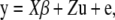
We applied our EMMA method to the same maize panel data consisting of 553 SNPs and three phenotypes across 277 diverse inbred lines (Flint-Garcia et al. 2005) analyzed with the current mixed-model implementations (Yu et al. 2006). We used the genotype similarity matrix defined in materials and methods as an additional variance component. Both the SAS and the TASSEL implementations of a unified mixed model (Yu et al. 2006) take nearly 2 hr for a single run over the flowering-time phenotype data set with Intel 2.8-GHz Dual Core CPU, and ASREML, which is known to be more efficient than SAS, takes 20 min (1201 sec) of running time. The execution time of our mixed-model implementation is substantially faster, taking only 2.6 min (157 sec). The comparison of the _P_-values obtained from the ASREML package and EMMA for flowering-time phenotypes shown in Figure 1a shows perfect concordance between the methods, suggesting that both methods provide the same accuracy. It should be noted that EMMA is much more efficient in spite of using orders of magnitude more of iterations to find the near global REML estimate using a grid search over the entire parameter space. EMMA also shows high stability of the numerical optimization procedure. In our results, TASSEL and ASREML implementations failed to provide _P_-values in 4 and 1 SNPs, respectively, of 553 SNPs, possibly due to the instability of the numerical optimization procedure, while EMMA succeeds for all the SNPs over all the data sets covered in this article.
Figure 1.—


(a) Direct comparison of _P_-values between ASREML and EMMA, computed from 553 SNPs of maize panel data and the flowering-time phenotype using a similarity-based kinship matrix. All _P_-values are almost identical, implying that two methods are almost identical in terms of accuracy. One SNP in ASREML failed to converge during the variance-component estimation while it succeeded in EMMA. (b) Cumulative distribution of _P_-values across different models. Under the assumption that the SNPs are unlinked and there few true SNP associations, the observed _P_-values are expected to be close to the cumulative _P_-values. A large deviation from the expectation implies that the statistical test may cause spurious associations. Simple, a simple _t_-test; SA, structured association; MM, an _F_-test with a mixed model with a specified kinship matrix.
Since the kinship matrix based on SPAGeDi software as suggested by the unified mixed model is not guaranteed to be positive semidefinite, we explore other ways to estimate the variance components due to genetic background. We use a genotype similarity matrix and a phylogenetic control matrix that guarantee positive semidefiniteness. Haplotype similarity matrices are not applicable to this data set due to sparse genotype density. We compared the goodness-of-fit of these kinship matrices in addition to the SPAGeDi-based kinship matrix over three maize phenotypes using the BIC, which provides a measure of how well each model fits the data. Adjusting for the sample size and the number of free parameters, Table 1 shows that the goodness-of-fits of the three kinship matrices based on maximum-likelihood estimates are comparable, while all of them were significantly better than not using a mixed model.
TABLE 1.
Goodness-of-fit of different models and kinship matrices in explaining phenotypic variation of maize quantitative traits
| Flowering time | Ear height | Ear diameter | |||||
|---|---|---|---|---|---|---|---|
| Method | Kinship matrix | −2 (ML) | BIC | −2 (ML) | BIC | −2 (ML) | BIC |
| Simple | NA | 1632.8 | 1643.9 | 2296.0 | 2307.1 | 1282.6 | 1293.5 |
| MM | SPAGeDi | 1524.3 | 1541.0 | 2237.7 | 2254.3 | 1254.2 | 1270.5 |
| MM | Genotype similarity | 1527.5 | 1544.2 | 2243.1 | 2259.8 | 1266.6 | 1282.9 |
| MM | Phylogenetic control | 1521.6 | 1538.6 | 2227.3 | 2243.9 | 1248.9 | 1265.2 |
| SA | NA | 1525.7 | 1547.9 | 2248.9 | 2271.1 | 1276.9 | 1298.7 |
| SA+MM | SPAGeDi | 1494.9 | 1522.7 | 2220.3 | 2248.1 | 1253.6 | 1280.8 |
| SA+MM | Genotype similarity | 1500.9 | 1528.7 | 2227.1 | 2254.9 | 1266.5 | 1293.7 |
| SA+MM | Phylogenetic control | 1491.6 | 1519.4 | 2213.2 | 2241.0 | 1248.2 | 1275.4 |
The cumulative _P_-value distribution seen in Figure 1b shows that the three kinship matrices correct for the inflated false positives significantly better than the simple linear model. As illustrated by previous studies, the cumulative distribution of _P_-values is expected to follow that of a uniform distribution with no inflated false positives because only a tiny fraction of all SNPs are expected to be true positives (Aranzana et al. 2005; Yu et al. 2006; Zhao et al. 2007). The genotype similarity matrix performs slightly better than the other two kinship matrices, especially for small _P_-values. Since the simpler kinship matrices show comparable or better goodness-of-fit and false positive reduction results while guaranteeing positive semidefiniteness, we apply only these simple kinship matrices in the following sections.
We also applied our EMMA method to perform genomewide association mapping of the flowering-time phenotype in which statistically significant associations are reported in previous studies. The cumulative distribution of _P_-values across 13,416 nonsingleton SNPs across 95 strains obtained from EMMA is shown in Figure 2a. The cumulative distribution of _P_-values with a haplotype similarity matrix nearly follows the expected distribution, implying that mixed models significantly outperform structured association in eliminating the inflation of false positives for this data set. Phylogenetic control reduces a large portion of inflated false positives, but residual inflation is still observed. Structured association and simple linear regression showed much larger inflation of false positives, consistent with the previous studies. After correction for genetic relatedness, the previously known FRI gene is still found to be significant at a nominal _P_-value of P = 10−5 across different kinship matrices. Our independent analyses are consistent with the more extensive results of Arabidopsis association mapping recently published (Zhao et al. 2007).
Figure 2.—


Genomewide cumulative distribution of observed _P_-values between (a) 13,416 Arabidopsis SNPs and flowering-time phenotypes across 95 strains using various models and(b) 106,040 mouse HapMap SNPs and three phenotypes, body weight (374 measurements over 38 strains), liver weight (304 measurements over 34 strains), and saccharin preference (280 measurements across 24 strains). S or Simple, a simple _t_-test; SA, structured association; MM, an _F_-test with a mixed model with a haplotype similarity kinship matrix; SA+MM, the unified mixed model using the output of STRUCTURE as additional fixed effects.
High-resolution genomewide association mapping in inbred mouse strains:
We performed a high-resolution genomewide association-mapping study using our mixed-model method over inbred mouse strains. We used the Broad mouse HapMap SNPs, containing nearly 140,000 SNPs expected to cover most of genetic variation among 48 inbred strains. For phenotypes, we used initial body weight and liver weight phenotypes downloaded from the Jackson Laboratory mouse phenome database (Jackson Laboratory 2004). In addition, we used a saccharin preference phenotype where statistically significant associations were identified in a previous study (Reed et al. 2004). Among 48 genotyped strains, 38, 34, and 24 strains had phenotype values available for body weight, liver weight, and saccharin preference, respectively. Each phenotype has on average 10 multiple measurements across different individual mice per strain.
The cumulative distributions of observed _P_-values in Figure 2 show that, without correcting for population structure, the rate of false positives is very high. In particular, the body weight phenotype has a substantial inflation of false positives. When our mixed model is used, the inflation of the statistics is significantly reduced in all three phenotypes.
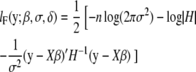
Figure 3 shows genomewide association signals for the three phenotypes. Comparing Figure 3a and 3b, it is obvious that, without correcting for population structure, many false positives are observed at a genomewide level of significance due to inflated _P_-values. Without correcting for population structure, we were able to identify nearly 6000 SNPs at a nominal _P_-value of 10−6 and 283 SNPs with _P_-values <10−10. However, none are significant after applying the mixed model. This strongly supports that most of the significant associations without correcting for population structure are indeed false positives. Interestingly, although the strongest signals for the body weight after applying the mixed model are not genomewide significant, they are concentrated in the region around 114 Mb in chromosome 8. This region almost exactly falls into the LOD peak of a previously known body weight QTL Bwq3 (Annuciado et al. 2001). The _P_-value of the most significant locus is 3.8 × 10⁻⁶ with the _F_-test, explaining 49% of the overall phenotypic variance and 39% of the phenotypic variation due to the genetic variance component. Although it is slightly below the genomewide significance threshold with a conservative Bonferroni correction, if utilizing the results from previous QTL studies, the locus can be declared as significant over the region of known body weight QTL.
Figure 3.—


Genomewide scans for association with initial body weight, liver weight, and saccharin preference, using simple _t_-tests and _F_-tests with mixed models, on the basis of a kinship inferred from haplotype similarities.
For the liver weight phenotype, we identified a genomewide significant association around the region of 34.5 Mb in chromosome 2. This falls into a previously known liver weight QTL Lvrq1 (Rocha et al. 2004). The region also contains many potentially relevant QTL such as organ weight (Orgwq2) (Leamy et al. 2002), spleen weight (Sp1q1) (Rocha et al. 2004), heart weight (Hrtq1) (Rocha et al. 2004), and lean body mass (Lbm1) (Masinde et al. 2002). The pointwise _P_-value of the most significant SNP was 1.2 × 10⁻⁹, which explains 59% of the genetic variance component. When comparing the genomewide _P_-values between the simple _t_-test and mixed models in Figure 3, c and d, we observe that the inflation of _P_-values is reduced, but the signals are even more significant around the significant SNP at chromosome 2. This demonstrates that mixed-model association mapping can not only reduce the inflated false positives, but also reveal significant associations that have remained unidentified using conventional statistical methods in the case when the associated SNP is not highly correlated with population structure.
For the saccharin preference phenotype, we were able to identify a SNP 30 kb away from the Tas1r3 gene that is perfectly correlated with the SNP previously reported to have significant association with the phenotype (Reed et al. 2004). It explains 51% of the genetic variance component, with a _P_-value of 1.0 × 10⁻⁵. The SNP is neither genomewide significant nor the most significant. We believe this is due to the limited power of the study with a small number of strains.
Power of inbred model organism association mapping:
We evaluated the statistical power of association mapping of inbred model organisms in two different ways. First, we simulated an additive effect of a causal SNP over the existing phenotypes for mouse, Arabidopsis, and maize strains, similar to previous studies. Such simulation studies evaluate the SNP effect on the power maintaining the existing correlation structure of phenotypes. However, they do not change the effect of the genetic background or the number of multiple measurements, and no random variable other than the SNP is involved in the power simulation. As an alternative model-driven method for simulation studies, we generated simulated phenotypes randomly sampled from a multivariate normal distribution with various effects of population structure on the phenotypic variation. A SNP effect is simulated on the randomly generated samples, and the statistical power is evaluated. In this way, we can simulate not only the SNP effect but also different genetic backgrounds and different numbers of replicated measurements. We believe that our simulation analysis provide a more extensive understanding of the statistical power of association mapping with model organisms.
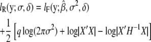
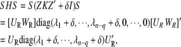
Figure 4 shows the statistical power with respect to the additive SNP effect on the Arabidopsis and maize flowering-time phenotypes and three inbred mouse phenotypes used in this article. The maize panel data set consisting of 277 strains has high statistical power, achieving 80% power with a SNP effect explaining 5% of phenotypic variation. Genomewide significance can also be achieved with high power with 10% of SNP effects. For the Arabidopsis data set consisting of 95 strains, the statistical power is decreased, and roughly twice the SNP effect would be needed compared to the maize panels to achieve the same statistical power. For the inbred mouse phenotypes, genomewide power is achievable only when the SNP explains a very large portion of phenotypic variance. In our results, the plausible significant associations explained >35% of the phenotypic variance. The power to achieve genomewide power is largely dependent on the number of available strains. Table 2 summarizes the most plausible associations in these three phenotypes.
Figure 4.—


Comparisons of the statistical power of the EMMA method across three different inbred mouse phenotypes and flowering time of Arabidopsis and maize, by randomly selecting causal SNPs across the genomewide SNPs. (a) Pointwise power denotes the power to identify causal SNPs at a nominal _P_-value of 0.05. (b) Regionwide power assumes 50 hypothetical tagSNPs in a genomic region. With 20 kb between tagSNPs, the genomic region covers up to 1 Mb. (c) Genomewide power is the power to achieve genomewide significance using the _P_-value threshold 10−5, which is conservative compared to the permutation-based genomewide significance thresholds using the original phenotypes. The phenotypic variation explained by SNP effect is computed assuming a minor allele frequency (MAF) of 0.3.
TABLE 2.
List of plausible associations in the mouse association mapping
| _P_-value | Variance explained (%) | ||||||||
|---|---|---|---|---|---|---|---|---|---|
| Phenotype | Chromosome | Position | _F_-test | LR test | Overall | Genetic | Alleles | MAF | Notes |
| Body weight | 8 | 113,588,970 | 3.9 × 10⁻⁶ | 1.9 × 10⁻⁵ | 49.0 | 38.7 | A/C | 0.27 | 300 kb from the LOD peak of Bwq3 QTL |
| Liver weight | 2 | 34,499,435 | 1.2 × 10⁻⁹ | 1.4 × 10⁻⁷ | 39.1 | 58.6 | G/C | 0.50 | Genomewide significant, within Lvrq1 QTL |
| Saccharin preference | 4 | 154,883,600 | 1.0 × 10⁻⁵ | 7.5 × 10⁻⁵ | 35.9 | 50.6 | G/A | 0.31 | 30 kb from Tas1r3 gene |
Next, we performed simulation studies by sampling phenotypes from multivariate normal distribution on the basis of the kinship matrix of 48 inbred mouse strains with different effects of genetic background due to population structure. We observed a significant increase of power when multiple measurements are used. Figure 5a shows the effect of multiple measurements on the statistical power when the variance from the genetic component and the residual component are the same. It suggests that using just a single measurement per strain may result in a significant decrease in power. Even though multiple measurements are used, if only the phenotypic mean is used in the analysis and the individual measurements are not taken into account, the statistical power would decrease significantly. Comparing Figure 5b with 5a clearly shows the advantage of using individual measurements over the phenotypic mean in the statistical analysis. It shows that the statistical power may differ by up to a factor of two between the two methods. Other mixed-model association-mapping studies use only the mean values in their analysis, not fully utilizing the potential of individual measurements.
Figure 5.—


Comparisons of the genomewide power of the EMMA method applied to inbred mouse associations for simulated phenotypes with various SNP effects, genetic background effects, and numbers of multiple measurements. The significance threshold is P = 10−5. t is the number of multiple measurements per strain, and  is the fraction of the variance explained by genetic background among overall phenotypic variances when the SNP effect is not added. (a) With
  varying β and t. (b) The same as a, using the mean phenotype value per strain instead of individual measurements. (c) With 10 multiple measurements per strain, varying β and
  (d) With β = σ, varying t and
  The effect of population structure is varied by changing the ratio of two variance components, and the numbers of multiple measurements are simulated with (a) 10 measurements and (b) a single measurement per strain.
Figure 5c shows that a large relative effect from genetic background reduces the statistical power. As the genetic background contributes a larger portion of phenotypic variance, the within-strain variance becomes smaller than the between-strain variance, and this limits the contribution of multiple measurements to the statistical power (Belknap 1998). For example, in an extreme case, when  the residual variance is zero and the replicated measurement does not increase the power since there is no variability of phenotype within strains.
Figure 5d shows more clearly the effect of genetic background and multiple measurements at a glance. When a SNP explains a fairly large fraction (17%) of phenotypic variance, the genomewide significance level can be achieved with high power only when the phenotype has very small population structure effect and the number of replicates is large. As the effect from genetic background becomes larger, the advantage of using multiple measurements decreases significantly.
DISCUSSION
In this article, we proposed an efficient statistical method to perform association mapping with structured samples on the basis of a linear mixed model. Our results with maize and Arabidopsis panels show that EMMA robustly reduces the inflated false positives under a structured population similar to currently available mixed-model implementations. The accuracy and stability of the numerical optimization in EMMA is greater than others due to global optimization of likelihood function and guaranteed convergence properties with a smaller search space. Our presentation of the EMMA method is focused on a particular case of a mixed model where two variance components are involved because this is the typical model that previous studies assume, and it is straightforward to correct population structure via one kinship matrix inferred from genomewide markers.
The computational efficiency of EMMA is orders of magnitude greater than that of other widely used implementations. When multiple measurements per strain are used across different individuals, the relative efficiency is further increased. This is of a great importance when the computational cost may be a bottleneck in the statistical analysis of high-throughput data such as genomewide gene expressions. For example, the single run of genomewide association mapping of mouse body weight phenotypes with multiple measurements would take up to a month of CPU time with other implementations, while EMMA takes only a single CPU hour. When hundreds and thousands of phenotypes are available such as in the analysis of whole-genome expression data, the computational cost of previous implementations is prohibitive even with high-performance computing. It should be noted that there are other techniques developed for improving computational efficiency of the numerical estimation in a more general context of linear mixed models such as average information REML (Gilmour et al. 1995), but these techniques would not provide us with the same improvements on the efficiency of each iterative procedure.
Our results of inbred mouse association mapping show the potential and limitations of genomewide inbred mouse association studies. It is remarkable that we were able to identify significant associations at a genomewide level without inflation of false positives, under the limited statistical power of the method. Although there is a possibility that residual confounding still remains with mixed-model association, we believe that the most significant SNP associated with liver weight is likely to be a true positive because it explains a large portion of phenotypic variations between the strains beyond genetic background effect so that the conservative Bonferroni-adjusted _P_-value still remains significant. The SNP associated with body weight looks also plausible, but it could possibly be due to residual confounding that is not completely captured by a kinship matrix. Likewise, other significant associations can possibly be due to residual confounding not captured by the kinship matrix, so the identified associations must be verified through independent analysis.
In a more general context of association mapping that requires the use of multiple variance components, the computational advantages of EMMA are not applicable since EMMA can effectively solve a model only with one correlated variance component. For example, when allowing heterozygous alleles for outbred individuals, the full model typically takes both additive and dominant variance components in the linear mixed model (Lynch and Ritland 1999; Arbelbide et al. 2006). Likewise, if strain-specific environmental random effects or other additional random effects are to be considered such as in plant association mapping, multiple variance components need to be used. In such cases where EMMA is not directly applicable, computational bottlenecks may be the biggest obstacles in analyzing large amounts of data such as genomewide expression profiles. EMMA can still be applied in this case if a reasonable approximation is combined with other standard mixed-model methods taking multiple variance components. Under the null hypothesis, it is possible to estimate the ratio between multiple variance components using the full model, and EMMA can be applied under an alternative hypothesis assuming that the ratio between variance components is preserved. Since variance-component estimation under the null hypothesis needs to be done once across a larger number of alternative hypotheses for each marker, such an approximation procedure provides a large amount of computational efficiency essentially equivalent to EMMA with one variance component. Although the approximated test may lose statistical power slightly, the false positive rates would not be inflated.
There have been several genomewide association-mapping studies with inbred mouse strains. To the best of our knowledge, our results are the first whole-genome association mapping of inbred mice that takes the genetic relatedness into account via a statistical method supported by asymptotic theory. Previous studies either do not take the population structure into account (Cervino et al. 2007) or apply heuristics to reduce the confounding effect from population structure. For example, the weighted version of the _F_-statistic (Pletcher et al. 2004) does not follow the asymptotic null distribution. Redefining the significance level on the basis of the empirical null distribution given the heritability parameter (Liu et al. 2006) or the weighted permutation (McClurg et al. 2007) rescales the _P_-values only similar to genomic control and will suffer from a lack of power as the genetic background effect becomes larger.
Our power simulation studies provide assistance to the design of the association study under the effect of population structure. Multiple factors are involved in determining the condition for identifying a locus, and it cannot be represented simply by a single value such as phenotypic variance explained by the SNP. Our results show the importance of multiple measurements of phenotypes from multiple animals for each strain and of directly using the individual measurements in the statistics for association mapping. Taking individual measurements into account within the association mapping is much more computationally intensive. EMMA provides a method for efficiently handling individual measurements. In addition, our results also demonstrate the effect of genetic background on the statistical power. As the population structure explains larger phenotypic variance, the power using multiple measurements becomes lower.
Our results show that phylogenetic control can control for population structure as effectively as the linear mixed model based on the genetic similarity matrix in some data sets despite the limited ability of the model to represent complex genetic relatedness. Since genetic similarity matrices are better models when accounting for recombination and hybridization, and also are easier to compute, phylogenetic control is not preferred in association mapping in model organisms. However, it is possible to compute the likelihood of the phylogenetic control model in linear time (Felsenstein 1985), and this may be useful when a very large number of individuals are to be tested.
Acknowledgments
H.K. is partially supported by a Samsung Scholarship, and N.Z. is partially supported by a Microsoft graduate fellowship. H.K., N.Z., and E.E. are partially supported by National Science Foundation grant nos. 0513612 and 0713455 and National Institutes of Health (NIH) grant no. 1K25HL080079. D.H. is supported by Microsoft Research. Part of this investigation was supported using the computing facility made possible by the Research Facilities Improvement Program grant no. C06 RR017588 awarded to the Whitaker Biomedical Engineering Institute and the Biomedical Technology Resource Centers Program grant no. P41 RR08605 awarded to the National Biomedical Computation Resource, University of California (San Diego), from the National Center for Research Resources, NIH. Additional computational resources were provided by the California Institute of Telecommunications and Information Technology (Calit2). The mouse HapMap project is supported by the National Human Genome Research Institute, NIH.
APPENDIX: DERIVATION OF RESTRICTED LIKELIHOOD AND ITS DERIVATIVES
A derivation of Equations 6 and 7 from Equations 2 and 3 is presented in Patterson and Thompson (1971) and Harville (1974). However, their derivation is not straightforward, and it needs to be clarified how exactly it is related to spectral decomposition. Here we describe a more detailed description of obtaining Equations 6 and 7.
Plugging in the optimal parameters  and
and  in Equation 2, it follows that
 |
(A1) |
|---|
From Equation 4, it is straightforward that  And R can be rewritten as follows:
 |
(A2) |
|---|
 |
(A3) |
|---|
 |
(A4) |
|---|
where P = I − X(X_′_H_−1_X)−1_X_′_H_−1.
It is straightforward to show that
 |
(A5) |
|---|
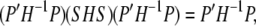 |
(A6) |
|---|
using the fact PS = S and SP = S. Consequently,
 |
(A7) |
|---|
where (·)+ denotes the pseudo-inverse of a matrix. Therefore, it follows that
 |
(A8) |
|---|
 |
(A9) |
|---|
 |
(A10) |
|---|
From Equations A1 and A10, it follows that
 |
(A11) |
|---|
The restricted likelihood of y is equivalent to computing the likelihood of Ay where S = _AA_′ and A_′_A = I:
 |
(A12) |
|---|
(Patterson and Thompson 1971; Harville 1974). On the other hand,
 |
(A13) |
|---|
Accordingly,  and
and  hold, and the restricted likelihood of y is equivalent to the likelihood of
  y ∼ N(0, σ2diag(λ_s_ + δ)). By plugging in
  to σ2, it immediately follows that
 |
(A14) |
|---|
References
- Annuciado, R. V. P., M. Nishimura, M. Mori, A. Ishikawa, S. Tanaka et al., 2001. Quantitative trait loci for body weight in the intercross between SM/J and A/J mice. Exp. Anim. 50 319–324. [DOI] [PubMed] [Google Scholar]
- Aranzana, M. J., S. Kim, K. Zhao, E. Bakker, M. Horton et al., 2005. Genome-wide association mapping in Arabidopsis identifies previously known flowering time and pathogen resistance genes. PLoS Genet. 1 e60. [DOI] [PMC free article] [PubMed] [Google Scholar]
- Arbelbide, M., J. Yu and R. Bernado, 2006. Power of mixed-model QTL mapping from phenotypic, pedigree and marker data in self-pollinated crops. Theor. Appl. Genet. 112 876–884. [DOI] [PubMed] [Google Scholar]
- Belknap, J. K., 1998. Effect of within-strain sample size on QTL detection and mapping using recombinant inbred mouse strains. Behav. Genet. 28 29–38. [DOI] [PubMed] [Google Scholar]
- Bhattacharya, T., M. Daniels, D. Heckerman, B. Foley, N. Frahm et al., 2007. Founder effects in the assessment of HIV polymorphisms and HLA allele associations. Science 315 1583–1586. [DOI] [PubMed] [Google Scholar]
- Bystrykh, L., E. Weersing, B. Dontje, S. Sutton, M. T. Pletcher et al., 2005. Uncovering regulatory pathways that affect hematopoietic stem cell using ‘genetical genomics’. Nat. Genet. 37 225–232. [DOI] [PubMed] [Google Scholar]
- Carlson, J. M., C. Kadie, S. Mallal and D. Heckerman, 2007. Leveraging hierarchical population structure in discrete association studies. PLoS One 2 e591. [DOI] [PMC free article] [PubMed] [Google Scholar]
- Casteele, T. V. D., P. Galbusera and E. Matthysen, 2001. A comparison of microsatellite-based pairwise relatedness estimators. Mol. Ecol. 10 1539–1549. [DOI] [PubMed] [Google Scholar]
- Cervino, A. C., A. Darvasi, M. Fallahi, C. C. Mader and N. F. Tsinoremas, 2007. An integrated in silico gene mapping strategy in inbred mice. Genetics 175 321–333. [DOI] [PMC free article] [PubMed] [Google Scholar]
- Crainiceanu, C. M., and D. Ruppert, 2004. Likelihood ratio tests in linear mixed models with one variance component. J. R. Stat. Soc. B 66 165–185. [Google Scholar]
- Dempster, A. P., D. B. Rubin and R. K. Tsutakawa, 1981. Estimation in covariance components models. J. Am. Stat. Assoc. 76 341–353. [Google Scholar]
- Devlin, B., and K. Roeder, 1999. Genomic control for association studies. Biometrics 55 997–1004. [DOI] [PubMed] [Google Scholar]
- Felsenstein, J., 1981. Evolutionary trees from dna sequences: a maximum likelihood approach. J. Mol. Evol. 17 368–376. [DOI] [PubMed] [Google Scholar]
- Felsenstein, J., 1985. Phylogenies and the comparative method. Am. Nat. 125 1–15. [Google Scholar]
- Felsenstein, J., and G. Churchill, 1996. A hidden Markov model approach to variation among sites in rate of evolution. Mol. Biol. Evol. 13 93–104. [DOI] [PubMed] [Google Scholar]
- Fitch, W., and E. Margoliash, 1967. The construction of phylogenetic trees—a generally applicable method utilizing estimates of the mutation distance obtained from cytochrome c sequences. Science 155 279–284. [DOI] [PubMed] [Google Scholar]
- Flint, J., W. Valdar, S. Shifman and R. Mott, 2005. Strategies for mapping and cloning quantitative trait genes in rodents. Nat. Rev. Genet. 6 271–286. [DOI] [PubMed] [Google Scholar]
- Flint-Garcia, S. A., A.-C. Thuillet, J. Yu, G. Pressoir, S. M. Romero et al., 2005. Maize association population: a high-resolution platform for quantitative trait locus dissection. Plant J. 44 1054–1064. [DOI] [PubMed] [Google Scholar]
- Frazer, K. A., E. Eskin, H. M. Kang, M. A. Bogue, D. A. Hinds et al., 2007. A sequence-based variation map of 8.27 million snps in inbred mouse strains. Nature 448 1050–1053. [DOI] [PubMed] [Google Scholar]
- Gilmour, A. R., R. Thompson and B. R. Cullis, 1995. Average information reml: an efficient algorithm for variance parameter estimation in linear mixed models. Biometrics 51 1440–1450. [Google Scholar]
- Graser, H. U., S. P. Smith and B. Tier, 1987. A derivative-free approach for estimating variance components in animal models by restricted maximum likelihood. J. Anim. Sci. 64 1362–1372. [Google Scholar]
- Gu, X., 2004. Statistical framework for phylogenomic analysis of gene family expression profiles. Genetics 167 531–542. [DOI] [PMC free article] [PubMed] [Google Scholar]
- Halperin, E., and E. Eskin, 2004. Haplotype reconstruction from genotype data using imperfect phylogeny. Bioinformatics 20 1842–1849. [DOI] [PubMed] [Google Scholar]
- Harville, D. A., 1974. Bayesian inference for variance components using only error contrasts. Biometrika 61 381–385. [Google Scholar]
- Henderson, C., 1984. Applications of Linear Models in Animal Breeding. University of Guelph, Guelph, ON, Canada.
- Jackson Laboratory, 2004. Mouse Phenome Database website. http://www.jax.org/phenome.
- Jander, G., S. R. Norris, S. D. Rounsley, D. F. Bush, I. M. Levin et al., 2002. Arabidopsis map-based cloning in the post-genome era. Plant Physiol. 129 440–450. [DOI] [PMC free article] [PubMed] [Google Scholar]
- Johnson, D. L., and R. Thompson, 1995. Restricted maximum likelihood estimation of variance components for univariate animal models using sparse matrix techniques and average information. J. Dairy Sci. 78 449–456. [Google Scholar]
- Kennedy, B. W., M. Quinton and J. A. van Arendonk, 1992. Estimation of effects of single genes on quantitative traits. J. Anim. Sci. 70 2000–2012. [DOI] [PubMed] [Google Scholar]
- Kishino, H., and M. Hasegawa, 1989. Evaluation of the maximum likelihood estimate of the evolutionary tree topologies from DNA sequence data, and the branching order in hominoidea. J. Mol. Evol. 29 170–179. [DOI] [PubMed] [Google Scholar]
- Leamy, L. J., D. Pomp, E. J. Eisen and J. M. Cheverud, 2002. Pleiotropy of quantitative trait loci for organ weights and limb bone lengths in mice. Physiol. Genomics 10 21–29. [DOI] [PubMed] [Google Scholar]
- Lindstrom, M. J., and D. M. Bates, 1988. Newton-Raphson and EM algorithms for linear mixed-effects models for repeated-measures data. J. Am. Stat. Assoc. 83 1014–1022. [Google Scholar]
- Liu, P., Y. Wang, H. Vikis, A. Maciaq, D. Wang et al., 2006. Candidate lung tumor susceptibility genes identified through whole-genome association analysis in inbred mice. Nat. Genet. 38 888–895. [DOI] [PubMed] [Google Scholar]
- Lynch, M., and K. Ritland, 1999. Estimation of pairwise relatedness with molecular markers. Genetics 152 1753–1766. [DOI] [PMC free article] [PubMed] [Google Scholar]
- Malosetti, M., C. G. van der Linden, B. Vosman and F. A. van Eeuwijk, 2007. A mixed-model approach to association mapping using pedigree information with an illustration of resistance to Phytophthora infestans in potato. Genetics 175 879–889. [DOI] [PMC free article] [PubMed] [Google Scholar]
- Martins, E. P., and T. F. Hansen, 1997. Phylogenetics and the comparative methods: a general approach to incorporating phylogenetic information into the analysis of interspecific data. Am. Nat. 149 646–667. [Google Scholar]
- Masinde, G. L., X. Li, W. Gu, H. Davidson, M. Hamilton-Ulland et al., 2002. Quantitative trait loci (QTL) for lean body mass and body length in MRL/MPJ and SJL/J F(2) mice. Funct. Integr. Genomics 2 98–104. [DOI] [PubMed] [Google Scholar]
- McClurg, P., J. Janes, C. Wu, D. L. Delano, J. R. Walker et al., 2007. Genomewide association analysis in diverse inbred mice: power and population structure. Genetics 176 675–683. [DOI] [PMC free article] [PubMed] [Google Scholar]
- Meyer, K., 1989. Restricted maximum likelihood to estimate variance components of animal models with several random effects using a derivative free algorthm. Genet. Sel. Evol. 21 318–340. [Google Scholar]
- Nelder, J. A., and R. Mead, 1965. A simplex method for function minimization. Comput. J. 7 308–313. [Google Scholar]
- Nievergelt, C. M., O. Libiger and N. J. Schork, 2007. Generalized analysis of molecular variance. PLoS Genet. 3 e51. [DOI] [PMC free article] [PubMed] [Google Scholar]
- Nordborg, M., T. T. Hu, Y. Ishino, J. Jhaveri, C. Toomajian et al., 2005. The pattern of polymorphism in Arabidopsis thaliana. PLoS Biol. 3 e196. [DOI] [PMC free article] [PubMed] [Google Scholar]
- Oakley, T. H., Z. Gu, E. Abouheif, N. H. Patel and W.-H. Li, 2005. Comparative methods for the analysis of gene-expression evolution: an example using yeast functional genomic data. Mol. Biol. Evol. 22 40–50. [DOI] [PubMed] [Google Scholar]
- Patterson, H. D., and R. Thompson, 1971. Recovery of inter-block information when block sizes are unequal. Biometrika 58 545–554. [Google Scholar]
- Patterson, N., A. Price and D. Reich, 2006. Population structure and eigenanalysis. PLoS Genet. 2 e190. [DOI] [PMC free article] [PubMed] [Google Scholar]
- Peter, L. L., R. F. Robledo, C. J. Bult, G. A. Churchill, B. J. Paigen et al., 2007. The mouse as a model for human biology: a resource guide for complex trait analysis. Nat. Rev. Genet. 8 58–69. [DOI] [PubMed] [Google Scholar]
- Piepho, H. P., 2001. A quick method for computing approximate thresholds for quantitative trait loci detection. Genetics 157 425–432. [DOI] [PMC free article] [PubMed] [Google Scholar]
- Pletcher, M., P. McClurg, S. Batalov, A. Su, S. Barnes et al., 2004. Use of a dense single nucleotide polymorphism map for in silico mapping in the mouse. PLoS Biol. 2 e393. [DOI] [PMC free article] [PubMed] [Google Scholar]
- Price, A., N. Patternson, R. Plenge, M. Weinblatt, N. Shadick et al., 2006. Principal components analysis corrects for stratification in genome-wide association studies. Nat. Genet. 38 904–909. [DOI] [PubMed] [Google Scholar]
- Pritchard, J., M. Stephens, N. Rosenberg and P. Donnelly, 2000. Association mapping in structured populations. Am. J. Hum. Genet. 67 170–181. [DOI] [PMC free article] [PubMed] [Google Scholar]
- Reed, D. R., S. Li, X. Li, L. Huang, M. G. Tordoff et al., 2004. Polymorphisms in the taste receptor gene (Tas1r3) region are associated with saccharin preference in 30 mouse strains. J. Neurosci. 24 938–946. [DOI] [PMC free article] [PubMed] [Google Scholar]
- Rocha, J., E. J. Eisen, L. Van Vleck and D. Pomp, 2004. A large-sample QTL study in mice: Ii. body composition. Mamm. Genome 15 100–113. [DOI] [PubMed] [Google Scholar]
- SAS Institute, 2004. SAS/STAT 9.1 User's Guide. SAS Institute, Cary, NC.
- Smith, S. P., 1990. Estimation of genetic parameters in non linear models, pp. 190–206 in Advances in Statistical Methods for Genetic Improvement of Livestock, edited by D. Gianola and K. Hammond. Springer-Verlag, New York.
- Storey, J. D., and R. Tibshirani, 2003. Statistical significance for genomewide studies. Proc. Nat. Acad. Sci. USA 100 9440–9445. [DOI] [PMC free article] [PubMed] [Google Scholar]
- Thomas, S. C., and W. G. Hill, 2000. Estimating quantitative genetic parameters using sibships reconstructed from marker data. Genetics 155 1961–1972. [DOI] [PMC free article] [PubMed] [Google Scholar]
- Wang, J., 2002. An estimator for pairwise relatedness using molecular markers. Genetics 160 1203–1215. [DOI] [PMC free article] [PubMed] [Google Scholar]
- Welham, S. J., and R. Thompson, 1997. Likelihood ratio tests for fixed model terms using residual maximum likelihood. J. R. Stat. Soc. B 59 701–714. [Google Scholar]
- Yu, J., G. Pressoir, W. Briggs, B. I. Vroh, M. Yamasaki et al., 2006. A unified mixed-model method for association mapping that accounts for multiple levels of relatedness. Nat. Genet. 38 203–208. [DOI] [PubMed] [Google Scholar]
- Zhao, K., M. J. Aranzana, S. Kim, C. Lister, C. Shindo, et al., 2007. An Arabidopsis example of association mapping in structured samples. PLoS Genet. 3 e4. [DOI] [PMC free article] [PubMed] [Google Scholar]
- Zou, F., J. A. Gelfond, D. C. Airey, L. Lu, K. F. Manly et al., 2005. Quantitative trait locus analysis using recombinant inbred intercrosses: theoretical and empirical considerations. Genetics 170 1299–1311. [DOI] [PMC free article] [PubMed] [Google Scholar]