Practical aspects of imputation-driven meta-analysis of genome-wide association studies (original) (raw)
Abstract
Motivated by the overwhelming success of genome-wide association studies, droves of researchers are working vigorously to exchange and to combine genetic data to expediently discover genetic risk factors for common human traits. The primary tools that fuel these new efforts are imputation, allowing researchers who have collected data on a diversity of genotype platforms to share data in a uniformly exchangeable format, and meta-analysis for pooling statistical support for a genotype–phenotype association. As many groups are forming collaborations to engage in these efforts, this review collects a series of guidelines, practical detail and learned experiences from a variety of individuals who have contributed to the subject.
INTRODUCTION
More than 100 validated susceptibility loci have now been identified through genome-wide association (GWA) studies of complex traits and common diseases. Often these discoveries have revealed new pathways involved in disease, but it is poorly understood for most associations which specific variants are causal, what is the biological mechanism, and how they interact with other genetic or environmental factors. Intensive follow-up work is required, beginning with targeted sequencing of these loci to obtain complete coverage of all genetic variation (common and rare) and to resolve independent signals of statistical association. What has become clear from these early successes of GWA studies is that the associated common variants at these loci have individually only modest effects, often with odds ratios of <1.2 for dichotomous traits, or with explained variance of <1% for quantitative traits. Also, a role for common variants with large effects can effectively be ruled out given adequate power of single studies to detect such effects and the relatively complete coverage of common variation of genome-wide single-nucleotide polymorphism (SNP) arrays (1,2). Large samples are required to discover the common variants with even smaller effects.
Collaborative efforts to combine the results from multiple studies range from informal comparisons of SNP associations to more comprehensive genome-wide meta-analyses. By increasing the effective sample size and power, these approaches are proving incredibly useful for gene discovery. For example, the Diabetes Genetics Initiative (DGI) (3), Wellcome Trust Case Control Consortium (WTCCC) (4), U.K. Type 2 Diabetes Genetics Consortium (UKT2DGC) (5), Finland-United States Investigation of NIDDM Genetics (FUSION) (6) compared their respective top hits and collectively demonstrated that some of these constituted bona fide associations with genome-wide significance (nominal P < 5 × 10⁻⁸). This work was subsequently extended to a formal meta-analysis of all GWA results generated by these studies (achieving a total sample size of ∼10 000), which led to the discovery of six additional risk loci (7), illustrating the value of meta-analysis across genome-wide studies led by different groups.
In addition to the meta-analysis in type 2 diabetes, we have recently been involved in similar collaborative efforts in bipolar disorder (8), rheumatoid arthritis (9), dyslipidemia (10), electrocardiographic QT interval duration (11) and multiple sclerosis, all resulting in the identification of novel associations. On the basis of our collective experiences, we review here some practical aspects of performing a meta-analysis and provide guidelines to facilitate future meta-analysis efforts. Ideally, one would like to combine raw genotype and phenotype data of multiple cohorts, thus allowing any test to be performed, including epistasis, gene-based tests and other phenotypes not originally considered. In practice, however, substantial restrictions (ethical, legal or otherwise) exist for sharing such data at the individual level. Recognizing such practical limitations, this review focuses on the scenario where individual groups perform data cleaning, genome-wide imputation of SNPs using HapMap and association testing (of main effects of single variants) independently, followed by exchange and meta-analysis of the generated association results.
Data cleaning and quality control
For genotype data, it would be hard to overstate the importance of data cleaning and quality control (12,13). Typical filtering steps for SNPs include missingness (call rate), differential missingness between cases and controls (for dichotomous traits), Hardy–Weinberg outliers (not in admixed populations) and the so-called plate-based technical artifacts (14). Individuals can be filtered based on missingness, heterozygosity (both may be due to poor DNA quality), cryptic relatedness and population structure (removing population outliers).
For phenotype data, we note that for quantitative traits, there must be explicit agreement on how the phenotype data should be normalized and coded in terms of scale and units (for example, QT interval duration may be reported on an absolute scale in milliseconds or as the number of standard deviations away from the population mean). These decisions are likely to vary by trait but should be made before the association analysis (and certainly before meta-analysis) is performed so that the effect estimates can be compared between studies.
To ensure consistent and uniform comparisons between studies, accurate annotation of the variant names and strand orientation is essential. We recommend explicit specification of the version of the human genome assembly (for example, NCBI build 35 or 36) and of dbSNP, and for each assay/polymorphism, the rs identifier in dbSNP, its chromosomal position (relative to the genome assembly), the alleles and their strand orientation (forward/+ or reverse/− strand of the genome assembly). This information is rarely necessary for the analysis of a single study, and is often neglected until a meta-analysis is performed. Comparison of polymorphisms between studies can sometimes be difficult as identifiers may change for the same polymorphism in different dbSNP releases, without a convenient way to convert them. Therefore, it is key to refer to a specific version of dbSNP to facilitate assay comparisons. Alignment of assay probe sequences against the human genome assembly should unambiguously determine the chromosomal position and orientation of variants.
In terms of strand orientation, we suggest that all SNPs have their alleles oriented on the forward/+ strand of NCBI build 36. For Affymetrix data, the publicly available NetAffx annotation files provide the necessary strand information (if not always error-free) to ‘flip’ alleles to the forward/+ strand. For example, rs4607103 (assay SNP_A-2091752 on the Affymetrix SNP 6.0 array) is a biallelic A/G SNP oriented on the reverse/− strand at position 64 686 944 on chr3 (build 36) near the ADAMTS9 gene (therefore, a T/C SNP on the positive/+ strand). Figuring out the strand orientation for SNPs on Illumina platforms is a little bit less straightforward, as the official annotation files do not refer to the absolute strand orientation of the assays relative to the human genome assembly. We would strongly encourage vendors to include accurate assay strand information with their platform annotations, or to develop convenient tools for such conversions. As a relatively straightforward solution (without having to align probe sequences), genotype data can be merged with HapMap data (where SNPs have a known orientation), and SNPs can be flipped if their alleles do not match those observed in HapMap. It is important to note that this will not work for A/T or C/G SNPs since they are complimentary bases (an A/T SNP cannot be distinguished from a T/A SNP). One might be able to reconcile some of these problematic SNPs based on a comparison with the observed allele frequencies in HapMap (though this might not work for very common SNPs with frequencies >0.40). Fortunately, Illumina platforms essentially exclude A/T and C/G SNPs, greatly simplifying an otherwise tedious flipping exercise (after removing a handful of A/T and C/G SNPs, if present). Also HapMap has various flavors (different genome builds, dbSNP releases and strand orientations), so it is important to keep track of which release is used (all releases up to 21a are based on NCBI build 35, and releases 22 and higher are based on build 36). Overall, we have found that these steps can be rate limiting (and perhaps the most frustrating). Although we have not extensively tested it ourselves, the IGG tool may offer some relief as it enables integration of data from Affymetrix and Illumina arrays with HapMap and export to various file formats (15).
Imputation and association testing
Individual studies often use genotyping platforms with different SNP content. One solution is to restrict the analysis to only those SNPs present on all platforms (for example, there are ∼250 000 overlapping SNPs on the Affymetrix SNP 6.0 and Illumina Human1M arrays), but this seems overly conservative. Alternatively, a number of tools including BIMBAM (16), IMPUTE (17), MACH (18) and PLINK (14) are now routinely used to impute the genotypes of the more than 2 million SNPs in HapMap based on the observed haplotype structure (19). These approaches allow studies to be analyzed across the same set of SNPs (directly genotyped and imputed) (7–9,11,20–24). By exploiting haplotype (multimarker) information, power is improved for untyped SNPs that were only poorly captured through pairwise linkage disequilibrium (LD), though this advantage is rather modest, especially for European populations (2,25). It is beyond the scope of this review to provide a comprehensive evaluation of these imputation methods (but we eagerly await a ‘bake-off’ of these approaches as part of the GAIN study (26)).
Genome-wide imputations require substantial computer power depending on the size of the study sample and of the reference panel (number of phased haplotypes in HapMap). Parallelization on a multi-node cluster can be achieved by splitting jobs up across chromosomes and into different sample subsets but keeping cases and controls together to avoid differential bias (27). Since NCBI build 36 (or UCSC hg18) has become the de facto standard for the human genome assembly, we recommend using the phased chromosomes of release 22, or the non-phased genotype data of the most current release (at time of writing, 23a). The performance with the phased haplotypes is expected to be better (if ever so slightly) than with unphased genotypes (28), but the key limitation of HapMap is its sample size (only 120 unique chromosomes in the European CEPH samples), affecting the accuracy of the imputation for less common variants. Therefore, we expect a significant improvement in performance with larger reference panels (such as HapMap Phase 3). Again, we stress that the strand orientation of the alleles must be consistent between genotype data and HapMap. Although imputation programs may protest when they encounter inconsistent allele names or observe large allele frequency differences, this will not catch all A/T or C/G SNPs on the reverse/− strand.
Not surprisingly, imputation is not perfect. Depending on the linkage disequilibrium between genotyped SNPs (used as input for the imputation) and untyped SNPs, some SNPs will be better predicted than others. For each imputed SNP in a given individual, imputation algorithms calculate posterior probabilities for the three possible genotypes (AA, AB, BB) as well as an effective allelic dosage (defined as the expected number of copies of a specified allele, ranging from 0 to 2). Even though imputation programs are able to produce ‘best-guess’ genotypes (those with the highest posterior probability), imputed genotypes cannot generally be treated as true (perfect) genotypes for association analysis. In fact, perhaps, the most important aspect of imputation is that the subsequent association analysis must take into account the uncertainty of the imputations, but there is no consensus on what is the best approach to do this.
One approach to minimize the effects of imputation error on association results is to restrict the analysis to SNPs genotyped on at least one platform (9,20). Another solution is to remove SNPs that are estimated to have poor imputation performance. One measure of imputation quality is the ratio of the empirically observed variance of the allele dosage to the expected binomial variance p(1 − p) at Hardy–Weinberg equilibrium, where p is the observed allele frequency from HapMap. When imputations have adequate information in predicting the unobserved genotypes from the observed haplotype backgrounds, this ratio should be distributed around unity, but collapses to zero as the observed variance of the allele dosage shrinks, reflecting progressively less information (more uncertainty). This follows the intuition that when this ratio is severely deflated (<1), genotypes of a given SNP exhibit only little variability across a sample, and there is only little information as to whether this SNP is associated with the phenotype. This ratio is equivalent to the RSQR_HAT value by MACH and the information content (INFO) measure by PLINK. In meta-analyses of height and type 2 diabetes, imputed SNPs were included only if the MACH RSQR_HAT > 0.3 (7,21). In a meta-analysis of bipolar disorder, imputed SNPs were analyzed if the PLINK information score is >0.8 (8).
Sophisticated Bayesian methods may offer better power than classical association tests (4,16,17,28). For example, the SNPTEST package offers a Bayesian test that can take into account the genotype uncertainty by sampling genotypes based on the estimated imputation probabilities and averaging the resulting Bayes Factors (4,17), though this is more computationally intensive than conventional likelihood ratio or score tests. Standard logistic or linear regression models can incorporate imputation uncertainty implicitly, where the standard error of the beta coefficient will reflect the uncertainty of the allele dosage. Furthermore, these models allow for the inclusion of covariates, and are widely available in standard statistics packages. SNPTEST also offers a logistic/linear regression function and calculates an information measure (PROPER_INFO), which is related to the effective sample size (power) for the genetic effect being estimated (4,17). In the recent type 2 diabetes meta-analysis, imputed SNPs were filtered out if this measure was <0.5 (7). We expect all these imputation certainty measures to be strongly correlated with one another.
Given the growing importance of shared control sample collections, we briefly note the dangers of combining cases genotyped on one platform and controls genotyped on another. To our knowledge, there are no studies that attempted to do imputation in order to be able to combine cases and controls in a single association study (and we certainly would not encourage that).
As many have advocated elsewhere, proper treatment of population structure is critical for GWA analysis (29,30). The PLINK package is widely used for matching cases to controls based on genotype information (identity-by-state, IBS), resulting in discrete strata of individuals that can be analyzed using the Cochran–Mantel–Haenszel test (14). Principal component analysis (PCA) using EIGENSTRAT is a powerful alternative to correct for population stratification (30), also providing functionality for removal of population sample outliers (in its helper routine SMARTPCA), and estimation of the number of statistically significant eigenvectors (only valid for homogenous, outbred populations) (31). Conveniently, the coordinates from EIGENSTRAT or from multi-dimensional scaling (MDS) analysis in PLINK along the first few axes of variation can be used as covariates for individuals in a linear/logistic regression framework, while allowing for uncertainty of imputed SNPs. We recommend that only genotyped SNPs with near-zero missingness be used for PCA-, MDS- or IBS-based matching.
After association analysis, it is critical to test the genome-wide distribution of the test statistic in comparison with the expected null distribution, specifically by calculating the genomic inflation factor λ and by making quantile–quantile (Q–Q) plots. The genomic inflation factor λ is defined as the ratio of the median of the empirically observed distribution of the test statistic to the expected median, thus quantifying the extent of the bulk inflation and the excess false positive rate (32). For example, the λ for a standard allelic test for association is based on the median (0.455) of the 1-d.f. χ2 distribution. Since λ scales with sample size, some have found it informative to report _λ_1000, the inflation factor for an equivalent study of 1000 cases and 1000 controls (33), which can be calculated by rescaling λ:
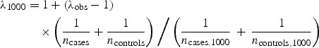
where _n_cases and _n_controls are the study sample size for cases and controls, respectively, and _n_cases,1000 and _n_controls,1000 are the target sample size (1000). The Q–Q plot is a useful visual tool to mark deviations of the observed distribution from the expected null distribution. As true associations reveal themselves as prominent departures from the null in the extreme tail of the distribution, we suggest that known associations (and their SNP proxies) are removed from the Q–Q plot in order to see if the null can be recovered. Inflated λ values or residual deviations in the Q–Q plot may point to undetected sample duplications, unknown familial relationships, a poorly calibrated test statistic, systematic technical bias or gross (uncorrected) population stratification (27), and need to be dealt with before performing meta-analysis. In addition, we encourage λ and Q–Q plots to be computed for genotyped and imputed SNPs separately to test for differences in their distribution properties.
We recommend that, prior to meta-analysis, the test statistic distributions be corrected for the observed inflation. Similarly, standard errors of beta coefficients should also be adjusted 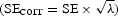 . Altogether, these steps help to ensure that association results are comparable and can be interpreted in a uniform way across studies.
Data exchange
The goal of data exchange is to follow an efficient procedure to exchange all information necessary for meta-analysis. Especially when collaborations involve large groups of investigators, it is critical to reach agreement as to which meta-analytical approaches and software tools will be used, and then to minimize the number of versions of each individual data set that need to be exchanged (requiring excellent version tracking and archiving). In our experience, it is useful to have at least two analysts work on the same data, preferably using different analysis tools, so that the results can be checked for consistency.
For exchanging GWA summary results, we propose that, at a minimum, the following data are exchanged for each SNP: rs identifier, chromosomal position (genome assembly and dbSNP versions must also be specified), coded allele, non-coded allele, frequency of the coded allele, strand orientation of the alleles, estimated odds ratio and 95% confidence interval of the coded allele (for dichotomous traits), beta coefficient and standard error (for linear/logistic regression modeling), _λ_-corrected _P_-value, call rate (for genotyped SNPs), ratio of the observed variance of the allele dosage to the empirically observed variance (for imputed SNPs) and average maximal posterior probability (for imputed SNPs). These data are sufficient to perform a meta-analysis, since risk alleles and direction of effect are unambiguously defined, even when individual studies used different genotyping platforms, imputation algorithms or association testing software.
For meta-analysis, it is critical that the estimated effect (odds ratio or beta) refers uniquely to the same allele (which we define as the ‘coded’ allele) across studies. Therefore, alleles may need to be flipped if the strand orientation is reverse/− (assuming all alleles are to be oriented on the forward/+ strand), and subsequently, coded and non-coded alleles may need to be swapped (and the direction of the odds ratio or sign of the beta flipped) to make both consistent across studies. Choice of the coded allele is, of course, arbitrary. One suggestion would be to use HapMap to define the coded allele as, for example, the observed minor allele. Using a pre-specified allele will help achieve consistency in the direction of effect between independent studies.
Meta-analysis
For dichotomous traits, _z_-scores can be calculated from the _λ_-corrected _P_-values for each study or directly from the test statistics (for example,  for 1-d.f. χ2 values), with the sign of the _z_-scores indicating direction of effect in that study (z > 0 for odds ratio >1). These _z_-scores can then be summed across multiple studies weighting them by the per-study sample size, as follows:
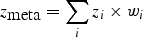
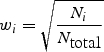
where z i is the _z_-score from study i, _w_i is the relative weight of study i based on its samples size N i, and _N_total is the total sample size of all studies. The squared weights should always sum to 1. To adjust for asymmetric case/control sample sizes in the type 2 diabetes meta-analysis (7), we used the Genetic Power Calculator (34) to estimate the non-centrality parameter (NCP) for the given asymmetric case/control sample size, and then iteratively determined the ‘effective’ (symmetric) case/control sample size that returns the same NCP. (We found this procedure to be quite robust for different genetic models.) To incorporate imputation uncertainty, the sample size N i can be scaled by the SNP information measure (RSQR_HAT from MACH, INFO from PLINK, or PROPER_INFO from SNPTEST) to appropriately ‘down-weight’ the contribution of a study where a particular SNP was poorly imputed, while maintaining complete information for accurately imputed SNPs in other studies.
For quantitative traits, we combine association evidence across studies by computing the pooled inverse variance-weighted beta coefficient, standard error and _z_-score, as follows:
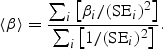
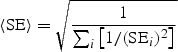
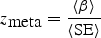
where β i and SE_i_ are the beta coefficient and standard error in study i, respectively. We emphasize that the units of the beta coefficients and standard errors must be the same across studies. It may be useful to compare the inverse variance-weighted _z_-score to an alternative _z_-score based on the (effective) sample size, which is computed as follows:
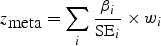
One potential advantage of using this _z_-score is that it allows the units of the beta coefficients and standard errors across studies to be different. Typically, the correlation between this _z_-score and the inverse variance-weighted _z_-score should be excellent (_r_2 > 0.99).
Interpretation
Once the meta-analysis _z_-scores are calculated, these can be converted into chi-square values (by squaring _z_-scores) and two-sided _P_-values (based on the normal distribution). The meta-analysis distribution must also be checked for inflation by computing λ and generating Q–Q plots (as we do for individual studies). Significant inflation of λ may indicate unknown sample duplications between different cohorts. Also, known associations can be conveniently used as a sanity check.
We have assumed that individual groups would perform data cleaning, imputation and analysis independently. As long as integrity of the data can be guaranteed (in terms of all recommendations we made here), we anticipate that a more ‘uniform’ meta-analysis standardized across all studies may not necessarily be better (powered) than a less formal meta-analysis of individual studies.
In the approaches outlined above, we focused primarily on the goal of association testing by pooling statistical support across studies using a fixed-effects model, not incorporating between-study heterogeneity and putting less emphasis on obtaining accurate pooled estimates of effect. In the presence of between-study heterogeneity, fixed-effects models are known to produce tighter confidence intervals and more significant _P_-values than random-effects models (35). Owing to limited sample size and power, however, individual GWA studies are likely to suffer from winner’s curse (overestimation of the true effect), causing variability in effect estimates by chance. Therefore, a random-effects model may well be too conservative compared with a fixed-effects model, especially when the primary goal is hypothesis testing and not effect estimation. Nevertheless, for meta-analyses across a large number of studies, it may be informative to test for heterogeneity by computing Cochran’s Q statistic as well as the _I_2 statistic and its 95% confidence interval (36). In some cases, study design differences can help explain apparent heterogeneity; see (37) for an insightful discussion about the _FTO-_obesity association discovered by WTCCC (38) and FUSION (6) but not DGI (3) (which had used BMI as one of the criteria to match cases to controls). We note that testing for between-study heterogeneity may also be useful for detecting allele flipping or strand problems.
Lastly, we need to be aware of the poor track record set by early genetic association studies (39). Therefore, we recommend strict adherence to a nominal _P_-value threshold of <5 × 10⁻⁸ to maintain a 5% genome-wide type I error rate, based on recent estimations of the genome-wide testing burden for common sequence variation (40,41). For populations with lower LD, stricter thresholds should be employed. Simulations based on resequencing data in the Yoruba sample from Ibadan, Nigeria (HapMap YRI), the total testing burden was estimated at two million independent tests (P < 2 × 10⁻⁸) (40).
We have made checklist of all critical decision points (Table 1) and developed a collection of programs called MANTEL for meta-analysis of GWA results, following the guidelines and methods presented here. These are available at http://www.broad.mit.edu/~debakker/meta.html. We also point the reader to the METAL software developed by Goncalo Abecasis, available at http://www.sph.umich.edu/csg/abecasis/metal/.
Table 1.
Meta-analysis check list
| Pre-exchange |
|---|
| Genome scan completed and ready for analysis? |
| Quality control (QC) steps performed on individual genome scan? |
| Individual QC: remove based on missingness, heterozygosity, relatedness, potential contamination, population outliers, and poorly genotyped samples [and other QC]? |
| SNP QC: remove based on missingness, Hardy–Weinberg, differential missingness, and plate-based association [as well as other QC]? |
| Population stratification estimated? |
| Analysis: genotyped SNPs |
| Analytical procedure controlling for |
| Population stratification? [Principal components, stratified (CMH) analysis, etc.] |
| Additional risk factors or covariates? |
| Analysis performed on genotyped SNPs? |
| Genomic inflation factor estimated? |
| _P_-values corrected for inflation? |
| Exchange file prepared? |
| Rs identifier |
| Chromosomal position |
| Strand orientation of allele (+/−) |
| Coded and noncoded allele |
| Allele frequency of the coded allele |
| Odds ratio |
| Beta and SE (for regression modeling) |
| Test statistic and _P_-value |
| Call rate |
| Imputation |
| HapMap release selected for imputation? |
| QC SNPs oriented to forward/+ strand and ordered to selected HapMap build? |
| Analysis: imputed SNPs |
| Analysis procedure on imputed SNPs |
| Accounts for genotype uncertainty? |
| Includes correction for population stratification? |
| Includes additional risk factors? |
| Analysis performed on imputed SNPs? |
| Removal of poorly imputed SNPs based on MACH R2 or SNPTEST criteria? |
| Genomic inflation factor estimated? |
| _P_-values corrected for inflation? |
| Exchange file prepared? |
| Rs identifier |
| Chromosomal position |
| Strand orientation of allele (+/−) |
| Coded and noncoded allele |
| Allele frequency of the coded allele |
| Odds ratio |
| Beta and SE (for regression modeling) |
| Test statistic and _P_-value |
| Ratio of the obs/exp variance of allele dosage |
| Average maximal posterior probability |
| Meta-analysis [weighted _z_-_score based_] |
| Individual study files collected, and version and date recorded? |
| Valid ranges for _P_-values, betas, SEs, test statistics? |
| Genome assembly versions specified? |
| dbSNP versions specified? |
| Strand orientation given for SNPs? |
| Effective sample sizes estimated from the data? |
| Individual study weights calculated from the data? |
| Study wide GC corrected _z_-score calculated from the data? |
| Results concordant with results generated by independent analyst? |
| For results of interest |
| Check that _z_-score directionality (i.e. risk) is consistent with observed (raw) data? |
| Estimate pooled odds ratios and confidence intervals from summary data (fixed-effects model or random-effects model)? |
| Calculate _I_2 and Q statistics to test for between-study heterogeneity? |
| Given observed heterogeneity, recalculate odds ratios (as necessary)? |
NOTE ADDED IN PROOF
The recent publication by Homer et al. describes a method to infer the presence of an individual's participation in a study based on summary allele frequency data (42). This has implications on data sharing policies, as it may compromise anonymity of study participation in certain cases. We strongly affirm that institutional guidelines must be adhered to with respect to privacy conditions when exchanging data.
FUNDING
S.R. is supported by a T32 NIH training grant (AR007530-23), an NIH K08 grant (KAR055688A), and through the BWH Rheumatology Fellowship program.
ACKNOWLEDGEMENTS
P.I.W.d.B. gratefully acknowledges the analysis group of the Cohorts for Heart and Aging Research in Genome Epidemiology (CHARGE) consortium for fruitful discussions about many of these issues.
Conflict of Interest statement. None declared.
REFERENCES
- 1.Barrett J.C., Cardon L.R. Evaluating coverage of genome-wide association studies. Nat. Genet. 2006;38:659–662. doi: 10.1038/ng1801. [DOI] [PubMed] [Google Scholar]
- 2.Pe’er I., de Bakker P.I.W., Maller J., Yelensky R., Altshuler D., Daly M.J. Evaluating and improving power in whole-genome association studies using fixed marker sets. Nat. Genet. 2006;38:663–667. doi: 10.1038/ng1816. [DOI] [PubMed] [Google Scholar]
- 3.Saxena R., Voight B.F., Lyssenko V., Burtt N.P., de Bakker P.I.W., Chen H., Roix J.J., Kathiresan S., Hirschhorn J.N., Daly M.J., et al. Genome-wide association analysis identifies loci for type 2 diabetes and triglyceride levels. Science. 2007;316:1331–1336. doi: 10.1126/science.1142358. [DOI] [PubMed] [Google Scholar]
- 4.Wellcome Trust Case Control Consortium. Genome-wide association study of 14,000 cases of seven common diseases and 3,000 shared controls. Nature. 2007;447:661–678. doi: 10.1038/nature05911. [DOI] [PMC free article] [PubMed] [Google Scholar]
- 5.Zeggini E., Weedon M.N., Lindgren C.M., Frayling T.M., Elliott K.S., Lango H., Timpson N.J., Perry J.R., Rayner N.W., Freathy R.M., et al. Replication of genome-wide association signals in UK samples reveals risk loci for type 2 diabetes. Science. 2007;316:1336–1341. doi: 10.1126/science.1142364. [DOI] [PMC free article] [PubMed] [Google Scholar]
- 6.Scott L.J., Mohlke K.L., Bonnycastle L.L., Willer C.J., Li Y., Duren W.L., Erdos M.R., Stringham H.M., Chines P.S., Jackson A.U., et al. A genome-wide association study of type 2 diabetes in Finns detects multiple susceptibility variants. Science. 2007;316:1341–1345. doi: 10.1126/science.1142382. [DOI] [PMC free article] [PubMed] [Google Scholar]
- 7.Zeggini E., Scott L.J., Saxena R., Voight B.F., Marchini J.L., Hu T., de Bakker P.I.W., Abecasis G.R., Almgren P., Andersen G., et al. Meta-analysis of genome-wide association data and large-scale replication identifies additional susceptibility loci for type 2 diabetes. Nat. Genet. 2008;40:638–645. doi: 10.1038/ng.120. [DOI] [PMC free article] [PubMed] [Google Scholar]
- 8.Ferreira M.A.R., O’Donovan M.C., Meng Y.A., Jones I.R., Ruderfer D.M., Jones L., Fan J., Kirov G., Perlis R.H., Green E.K., et al. Collaborative genome-wide association analysis supports a role for ANK3 and CACNA1C in bipolar disorder. Nat. Genet. 2008;40:1056–1058. doi: 10.1038/ng.209. [DOI] [PMC free article] [PubMed] [Google Scholar]
- 9.Raychaudhuri S., Remmers E.F., Lee A.T., Hackett R., Guiducci C., Burtt N.P., Gianniny L., Korman B.D., Padyukov L., Kurreeman F.A.S., et al. Common variants at CD40 and other loci confer risk of rheumatoid arthritis. Nat. Genet. 2008 doi: 10.1038/ng.233. in press, doi:10.1038/ng.233. [DOI] [PMC free article] [PubMed] [Google Scholar]
- 10.Kathiresan S., Willer C.J., Peloso G., Demissie S., Musunru K., Schadt E., Kaplan L., Bennett D., Li Y., Tanaka T., et al. Common DNA sequence variants at twenty-nine genetic loci contribute to polygenic dyslipidemia. Nat. Genet. 2008 doi: 10.1038/ng.291. in press. [DOI] [PMC free article] [PubMed] [Google Scholar]
- 11.Newton-Cheh C., Eijgelsheim M., Rice K., de Bakker P.I.W., Yin X., Estrada K., Bis J., Marciante K., Rivadeneira F., Noseworthy P.A., et al. Common variants at ten loci influence myocardial repolarization: the QTGEN consortium. Nat. Genet. 2008 doi: 10.1038/ng.364. in press. [DOI] [PMC free article] [PubMed] [Google Scholar]
- 12.Chanock S.J., Manolio T., Boehnke M., Boerwinkle E., Hunter D.J., Thomas G., Hirschhorn J.N., Abecasis G., Altshuler D., Bailey-Wilson J.E., et al. Replicating genotype–phenotype associations. Nature. 2007;447:655–660. doi: 10.1038/447655a. [DOI] [PubMed] [Google Scholar]
- 13.Neale B.M., Purcell S. The positives, protocols, and perils of genome-wide association. Am. J. Med. Genet. B Neuropsychiatr. Genet. 2008 doi: 10.1002/ajmg.b.30747. in press, doi:10.1002/ajmg.b.30747. [DOI] [PubMed] [Google Scholar]
- 14.Purcell S., Neale B., Todd-Brown K., Thomas L., Ferreira M.A., Bender D., Maller J., Sklar P., de Bakker P.I.W., Daly M.J., et al. PLINK: a tool set for whole-genome association and population-based linkage analyses. Am. J. Hum. Genet. 2007;81:559–575. doi: 10.1086/519795. [DOI] [PMC free article] [PubMed] [Google Scholar]
- 15.Li M.X., Jiang L., Ho S.L., Song Y.Q., Sham P.C. IGG: a tool to integrate GeneChips for genetic studies. Bioinformatics. 2007;23:3105–3107. doi: 10.1093/bioinformatics/btm458. [DOI] [PubMed] [Google Scholar]
- 16.Servin B., Stephens M. Imputation-based analysis of association studies: candidate regions and quantitative traits. PLoS Genet. 2007;3:e114. doi: 10.1371/journal.pgen.0030114. [DOI] [PMC free article] [PubMed] [Google Scholar]
- 17.Marchini J., Howie B., Myers S., McVean G., Donnelly P. A new multipoint method for genome-wide association studies by imputation of genotypes. Nat. Genet. 2007;39:906–913. doi: 10.1038/ng2088. [DOI] [PubMed] [Google Scholar]
- 18.Li Y., Abecasis G.R. MACH 1.0: rapid haplotype reconstruction and missing genotype inference. Am. J. Hum. Genet. 2006;S79:2290. [Google Scholar]
- 19.International HapMap Consortium. A second generation human haplotype map of over 3.1 million SNPs. Nature. 2007;449:851–861. doi: 10.1038/nature06258. [DOI] [PMC free article] [PubMed] [Google Scholar]
- 20.Barrett J.C., Hansoul S., Nicolae D.L., Cho J.H., Duerr R.H., Rioux J.D., Brant S.R., Silverberg M.S., Taylor K.D., Barmada M.M., et al. Genome-wide association defines more than 30 distinct susceptibility loci for Crohn’s disease. Nat. Genet. 2008;40:955–962. doi: 10.1038/NG.175. [DOI] [PMC free article] [PubMed] [Google Scholar]
- 21.Lettre G., Jackson A.U., Gieger C., Schumacher F.R., Berndt S.I., Sanna S., Eyheramendy S., Voight B.F., Butler J.L., Guiducci C., et al. Identification of ten loci associated with height highlights new biological pathways in human growth. Nat. Genet. 2008;40:584–591. doi: 10.1038/ng.125. [DOI] [PMC free article] [PubMed] [Google Scholar]
- 22.Willer C.J., Sanna S., Jackson A.U., Scuteri A., Bonnycastle L.L., Clarke R., Heath S.C., Timpson N.J., Najjar S.S., Stringham H.M., et al. Newly identified loci that influence lipid concentrations and risk of coronary artery disease. Nat. Genet. 2008;40:161–169. doi: 10.1038/ng.76. [DOI] [PMC free article] [PubMed] [Google Scholar]
- 23.Sanna S., Jackson A.U., Nagaraja R., Willer C.J., Chen W.M., Bonnycastle L.L., Shen H., Timpson N., Lettre G., Usala G., et al. Common variants in the GDF5-UQCC region are associated with variation in human height. Nat. Genet. 2008;40:198–203. doi: 10.1038/ng.74. [DOI] [PMC free article] [PubMed] [Google Scholar]
- 24.Chen W.M., Erdos M.R., Jackson A.U., Saxena R., Sanna S., Silver K.D., Timpson N.J., Hansen T., Orru M., Grazia Piras M., et al. Variations in the G6PC2/ABCB11 genomic region are associated with fasting glucose levels. J. Clin. Invest. 2008;118:2620–2628. doi: 10.1172/JCI34566. [DOI] [PMC free article] [PubMed] [Google Scholar]
- 25.Anderson C.A., Pettersson F.H., Barrett J.C., Zhuang J.J., Ragoussis J., Cardon L.R., Morris A.P. Evaluating the effects of imputation on the power, coverage, and cost efficiency of genome-wide SNP platforms. Am. J. Hum. Genet. 2008;83:112–119. doi: 10.1016/j.ajhg.2008.06.008. [DOI] [PMC free article] [PubMed] [Google Scholar]
- 26.Manolio T.A., Rodriguez L.L., Brooks L., Abecasis G., Ballinger D., Daly M., Donnelly P., Faraone S.V., Frazer K., Gabriel S., et al. New models of collaboration in genome-wide association studies: the Genetic Association Information Network. Nat. Genet. 2007;39:1045–1051. doi: 10.1038/ng2127. [DOI] [PubMed] [Google Scholar]
- 27.Clayton D.G., Walker N.M., Smyth D.J., Pask R., Cooper J.D., Maier L.M., Smink L.J., Lam A.C., Ovington N.R., Stevens H.E., et al. Population structure, differential bias and genomic control in a large-scale, case–control association study. Nat. Genet. 2005;37:1243–1246. doi: 10.1038/ng1653. [DOI] [PubMed] [Google Scholar]
- 28.Guan Y., Stephens M. Practical issues in imputation-based association mapping. 2008 doi: 10.1371/journal.pgen.1000279. http://quartus.uchicago.edu/~yguan/bimbam/resource/piBIMBAM.pdf . [DOI] [PMC free article] [PubMed] [Google Scholar]
- 29.Campbell C.D., Ogburn E.L., Lunetta K.L., Lyon H.N., Freedman M.L., Groop L.C., Altshuler D., Ardlie K.G., Hirschhorn J.N. Demonstrating stratification in a European American population. Nat. Genet. 2005;37:868–872. doi: 10.1038/ng1607. [DOI] [PubMed] [Google Scholar]
- 30.Price A.L., Patterson N.J., Plenge R.M., Weinblatt M.E., Shadick N.A., Reich D. Principal components analysis corrects for stratification in genome-wide association studies. Nat. Genet. 2006;38:904–909. doi: 10.1038/ng1847. [DOI] [PubMed] [Google Scholar]
- 31.Patterson N., Price A.L., Reich D. Population structure and eigenanalysis. PLoS Genet. 2006;2:e190. doi: 10.1371/journal.pgen.0020190. [DOI] [PMC free article] [PubMed] [Google Scholar]
- 32.Devlin B., Roeder K. Genomic control for association studies. Biometrics. 1999;55:997–1004. doi: 10.1111/j.0006-341x.1999.00997.x. [DOI] [PubMed] [Google Scholar]
- 33.Freedman M.L., Reich D., Penney K.L., McDonald G.J., Mignault A.A., Patterson N., Gabriel S.B., Topol E.J., Smoller J.W., Pato C.N., et al. Assessing the impact of population stratification on genetic association studies. Nat. Genet. 2004;36:388–393. doi: 10.1038/ng1333. [DOI] [PubMed] [Google Scholar]
- 34.Purcell S., Cherny S.S., Sham P.C. Genetic Power Calculator: design of linkage and association genetic mapping studies of complex traits. Bioinformatics. 2003;19:149–150. doi: 10.1093/bioinformatics/19.1.149. [DOI] [PubMed] [Google Scholar]
- 35.Kavvoura F.K., Ioannidis J.P. Methods for meta-analysis in genetic association studies: a review of their potential and pitfalls. Hum. Genet. 2008;123:1–14. doi: 10.1007/s00439-007-0445-9. [DOI] [PubMed] [Google Scholar]
- 36.Ioannidis J.P., Patsopoulos N.A., Evangelou E. Uncertainty in heterogeneity estimates in meta-analyses. Br. Med. J. 2007;335:914–916. doi: 10.1136/bmj.39343.408449.80. [DOI] [PMC free article] [PubMed] [Google Scholar]
- 37.Ioannidis J.P., Patsopoulos N.A., Evangelou E. Heterogeneity in meta-analyses of genome-wide association investigations. PLoS ONE. 2007;2:e841. doi: 10.1371/journal.pone.0000841. [DOI] [PMC free article] [PubMed] [Google Scholar]
- 38.Frayling T.M., Timpson N.J., Weedon M.N., Zeggini E., Freathy R.M., Lindgren C.M., Perry J.R., Elliott K.S., Lango H., Rayner N.W., et al. A common variant in the FTO gene is associated with body mass index and predisposes to childhood and adult obesity. Science. 2007;316:889–894. doi: 10.1126/science.1141634. [DOI] [PMC free article] [PubMed] [Google Scholar]
- 39.Hirschhorn J.N., Lohmueller K., Byrne E., Hirschhorn K. A comprehensive review of genetic association studies. Genet. Med. 2002;4:45–61. doi: 10.1097/00125817-200203000-00002. [DOI] [PubMed] [Google Scholar]
- 40.Pe’er I., Yelensky R., Altshuler D., Daly M.J. Estimation of the multiple testing burden for genomewide association studies of nearly all common variants. Genet. Epidemiol. 2008;32:381–385. doi: 10.1002/gepi.20303. [DOI] [PubMed] [Google Scholar]
- 41.Dudbridge F., Gusnanto A. Estimation of significance thresholds for genomewide association scans. Genet. Epidemiol. 2008;32:2227–234. doi: 10.1002/gepi.20297. [DOI] [PMC free article] [PubMed] [Google Scholar]
- 42.Homer T., Szelinger S., Redman M., Duggan D., Tembe W., Muehling J., Pearson J.V., Stephan D.A., Nelson S.F., Craig D.W. Resolving individuals contributing trace amounts of DNA to highly complex mixtures using high-density SNP genotyping microarrays. PLoS Genet. 2008;4:e1000167. doi: 10.1371/journal.pgen.1000167. [DOI] [PMC free article] [PubMed] [Google Scholar]