A statistical sampling algorithm for RNA secondary structure prediction (original) (raw)
Abstract
An RNA molecule, particularly a long-chain mRNA, may exist as a population of structures. Further more, multiple structures have been demonstrated to play important functional roles. Thus, a representation of the ensemble of probable structures is of interest. We present a statistical algorithm to sample rigorously and exactly from the Boltzmann ensemble of secondary structures. The forward step of the algorithm computes the equilibrium partition functions of RNA secondary structures with recent thermodynamic parameters. Using conditional probabilities computed with the partition functions in a recursive sampling process, the backward step of the algorithm quickly generates a statistically representative sample of structures. With cubic run time for the forward step, quadratic run time in the worst case for the sampling step, and quadratic storage, the algorithm is efficient for broad applicability. We demonstrate that, by classifying sampled structures, the algorithm enables a statistical delineation and representation of the Boltzmann ensemble. Applications of the algorithm show that alternative biological structures are revealed through sampling. Statistical sampling provides a means to estimate the probability of any structural motif, with or without constraints. For example, the algorithm enables probability profiling of single-stranded regions in RNA secondary structure. Probability profiling for specific loop types is also illustrated. By overlaying probability profiles, a mutual accessibility plot can be displayed for predicting RNA:RNA interactions. Boltzmann probability-weighted density of states and free energy distributions of sampled structures can be readily computed. We show that a sample of moderate size from the ensemble of an enormous number of possible structures is sufficient to guarantee statistical reproducibility in the estimates of typical sampling statistics. Our applications suggest that the sampling algorithm may be well suited to prediction of mRNA structure and target accessibility. The algorithm is applicable to the rational design of small interfering RNAs (siRNAs), antisense oligonucleotides, and _trans_-cleaving ribozymes in gene knock-down studies.
INTRODUCTION
RNA molecules participate in a variety of important biological processes that include catalysis, RNA splicing, regulation of transcription, translation, and RNA:DNA, RNA:RNA and RNA:protein interactions. The function of an RNA molecule is determined by its structure. However, it is extremely difficult to crystallize large RNA molecules for structural determination. Crystal structure has been determined only for a small number of RNA molecules, although exciting progress has been made for rRNAs in recent years (1). Secondary structures are highly conserved in evolution for most functional RNAs, e.g. tRNAs (2). On the other hand, RNA tertiary structural motifs involve interactions between secondary structure elements. To a large extent, RNA folding is driven by secondary structural features. For these reasons, elucidation of RNA secondary structure is an important step toward determination of three-dimensional structure and function of an RNA. Computational methods are valuable, because determination of secondary structure, particularly for long-chain RNA molecules, is difficult by experimental means.
From the perspective of statistical mechanics, characterization of the full ensemble of secondary structures for a given RNA sequence is of great interest (3,4). For example, an mRNA may exist as a population of different structures (5). On the other hand, multiple structures are known to be involved in a variety of RNA regulatory functions. These include the functioning of the 5S rRNA during prokaryotic protein synthesis (6,7), regulation of translation initiation in prokaryotes (8,9), and attenuation of transcription in enteric bacteria (10).
Free energy minimization is the most popular method for the prediction of RNA secondary structure from a single sequence. Although free energy models for secondary structure motifs have undergone refinements for more accurate characterization of folding thermodynamics, there is still uncertainty in the experimental estimates of the parameters. The free energy computed for a structure is an approximation as well, because of the assumption of free energy additivity and the need to extrapolate to loop sequences and loop sizes in the absence of measured estimates. Slight deviations in the free energy parameters can lead to substantial differences in the computed optimal folding. This ill conditioning of the RNA folding problem by free energy minimization has been well noted (11). Furthermore, the stability of secondary structure motifs can be affected by potential tertiary interactions that are unaccounted for in secondary structure prediction, and little is known about the thermodynamic contributions of tertiary motifs. Hence, the minimum free energy (MFE) structure derived from a folding algorithm may not be the true structure, and the true structure may be a suboptimal folding. These considerations provide additional motivations for us to more fully explore the ensemble of all secondary structures. Existing algorithms have only partially addressed the ensemble. We discuss below three major solutions that have been described.
First, mathematical algorithms (12,13) can predict optimal folding and can present a designed set of suboptimal foldings within any prescribed P% (0 ≤ P ≤ 100) of the MFE. The suboptimal algorithm is efficient for mitigating the uncertainties in the predictions; however, it has limitations. For each admissible base pair, the suboptimal algorithm generates the constrained optimal folding, with this pair as the constraint. Thus, it will regenerate the optimal folding if a base pair in the optimal folding is the constraint. For a sequence of n nucleotides, and _n_0 base pairs in the optimal folding, at most n(n – 1)/2 – _n_0 suboptimal foldings are examined by this algorithm. This set is common for all choices of P, and those within P% of the MFE are returned by the algorithm. For large P and for even moderate n, this is a small subset of all the suboptimal foldings within P% of the MFE because, as P increases, the number of all suboptimal foldings increases exponentially with n. Furthermore, if the least stable structure from this set is Q% away from the MFE, then for P < Q, no new suboptimal foldings are produced. A structure that is not one of the constrained optimal foldings generated by its base pairs is in the complementary set of the ‘missing’ suboptimal foldings, i.e. the collection of suboptimal foldings excluded by the suboptimal algorithm. For example, structures specified by removal of one or more base pairs from the optimal folding fall into this set.
Secondly, a recent mathematical algorithm deals with the computation of all suboptimal foldings within any specified increment of the MFE (14), and thus does comprehensively address the issue of ensemble. This represents a more analytical treatment than an earlier attempt (15). However, for this algorithm, because the number of suboptimal foldings grows exponentially, the run time shows an exponential behavior, as the range of the energy interval increases (14). Thus, even for moderate sequence length and moderate free energy interval, enumeration and examination of this huge set of suboptimal foldings become prohibitive.
Thirdly, the calculation of equilibrium partition functions and base-pairing probabilities (3) is an important advance toward the characterization of the Boltzmann ensemble of secondary structures. However, this elegant algorithm does not generate any secondary structures.
The dilemma, that the presentation of suboptimal foldings through a designed set is limited, whereas complete enumeration and examination of suboptimal foldings is difficult, appears to be very hard to resolve by a mathematical treatment. However, as we suggested with prototype algorithms (16,17), the generation of a statistically representative sample of secondary structures may provide a resolution to this dilemma. Here we describe a secondary structure sampling algorithm that incorporates comprehensive structural features and the recent thermodynamic parameters. We show that the algorithm generates a sample that is guaranteed to be representative. We present applications of the algorithm to illustrate statistical characterization and representation of the Boltzmann ensemble of secondary structures. Also, we illustrate how the algorithm can be employed in predictions of accessible target regions for rational design of RNA-targeting nucleic acids.
ALGORITHM
For an RNA molecule, the secondary structures in the Boltzmann ensemble are not all equally probable. The Boltzmann equilibrium probability of a secondary structure I for a sequence S is given by
P(I) = exp[–E(S, I)/_RT_]/U 1
where E(S, I) is the free energy of the structure for the sequence, R is the gas constant, T is the absolute temperature and U is the partition function for all admissible secondary structures of the RNA sequence, i.e. U = Σ_I_ exp[–E(S, I)/_RT_]. The Boltzmann equilibrium probability distribution gives the probability for every structure, and therefore statistically characterizes the ensemble. However, neither complete enumeration nor usual statistical sampling from a discrete distribution is feasible in this context, because the number of secondary structures grows exponentially with increasing length of the sequence. Here we describe a recursive algorithm that draws a representative sample from the Boltzmann equilibrium distribution.
The algorithm has two basic steps. Its forward step computes equilibrium partition functions for all substrings of an RNA sequence based on recent free energy parameters (18,19). The backward step takes the form of a recursive sampling algorithm to randomly draw secondary structures according to their probabilities given by equation 1. The equilibrium partition functions are used for calculating conditional sampling probabilities. By applying the algorithm to biological RNA sequences of a wide range of length, we demonstrate that a statistically representative sample of secondary structures can be quickly generated after the calculation of the partition functions.
Computing equilibrium partition functions
For an RNA molecule of n ribonucleotides, let the sequence fragment from the _i_th ribonucleotide from the 5′ end to the j_th ribonucleotide be denoted by R ij = r i r i +1 …_r j, 1 ≤ i, j ≤ n, where r i = A, C, G or U. Let I ij be a secondary structure on R ij that meets the usual constraints of unknotted structure and at least three intervening bases between any base pair. For structures under the constraints, let IP ij be a structure on R ij with the ends constrained to form a base pair. By summing over all structures on the fragment, the equilibrium partition functions restricted to R ij are defined as:
u(i, j) = Σ_Iij_ exp[–E(R ij, I ij )/_RT_] 2
up(i, j) = Σ_IPij_ exp[–E(R ij, IP ij )/_RT_] 3
where the sum for u(i, j) is over all possible I ij, and the sum for up(i, j) is over all possible IP ij. E(R ij, I ij ) is the free energy of structure I ij for R ij, and for the gas constant R and the absolute temperature T = 310.15 K, kcal/mol/RT = 1.6225. E(R ij, IP ij ) is the free energy of structure IP ij. Recursive calculation of partition functions was previously employed for computing base-pairing probabilities (3). The recursions in the Appendix extend this early work by including all but coaxial stacking from the recent free energy parameters (18,19). In particular, free energies for dangling ends have been incorporated. More specifically, the free energy rules and parameters include free energies for stacking in a helix, stacking for a terminal mismatch in a hairpin loop (size ≥ 4 nt) or an interior loop, and penalties for hairpin, bulge, interior and multibranched loops. Free energies for dangling ends are used for exterior and multibranched loops. For hairpins, a bonus for UU and GA first mismatches (included in the terminal stacking data) and a bonus for G_·_U closure preceded by two G nucleotides in base pairs are applied, and a penalty for oligo-C loops (all unpaired nucleotides are C) is used. A table is consulted for tetraloops with four unpaired nucleotides. For a bulge of 1 nt, the stacking energy of the adjacent pairs is added. For interior loops, tables for 1 × 1, 1 × 2 and 2 × 2 loops are consulted, and a penalty for asymmetry is applied. A terminal A_–_U, G_·_U penalty is explicitly applied to exterior loop, multibranched loops, bulges longer than 1 nt and triloops (hairpin loops with three unpaired nucleotides), while this penalty is included in the terminal stacking data for hairpin loops (size ≥ 4 nt) and interior loops. The free energy parameters are for 37°C and 1 M Na+; however, this algorithm can be used with any set of nearest-neighbor parameters derived for other conditions. The recursions for partition functions are presented in such a fashion that sampling probabilities can be readily derived.
With the partition function u(1, n) available, the Boltzmann equilibrium probability for a secondary structure _I_1 n of sequence _R_1 n can then be computed. Under the Boltzmann model, _I_1 n is a random variable. When _R_1 n is also considered a random variable, the Boltzmann equilibrium probability is, in fact, a conditional probability of the secondary structure, given the sequence data:
P(_I_1 n |_R_1 n ) = exp[–E(_R_1 n, _I_1 n )/_RT_]/u(1, n) 4
Sampling structures from the Boltzmann equilibrium probability distribution
In this section, we first present equations for computing sampling probabilities. Next, we describe the sampling algorithm. At the end, we discuss the features of the sampling algorithm, and illustrate them with examples.
Equations for computation of sampling probabilities. We previously described sampling algorithms for RNA secondary structures using a stacking energy model (16,17). The task of structure sampling can also be accomplished for a more comprehensive energy model, because the recursions for restricted partition functions correspond to sampling probabilities for mutually exclusive and exhaustive cases:
Sampling probability for a case = contribution to partition function by the case/partition function.
Specifically, consider a fragment R ij for which it is unknown whether the ends form a pair. For the five cases (a), (b), (c), (d) and (e) as shown in Figure A2 A2 in the derivation of the recursion for u(i, j) (equation A1 in the Appendix), the sampling probabilities are given by the following equations:
_P_0 = 1/u(i, j)
P ij = up(i, j)exp[–etp(i, j)/_RT_]/u(i, j)
P hj = up(h, j)exp{–[_ed_5(h, j, h – 1) + etp(h, j)]/RT}/u(i, j), i < h < j,
P il = up(i, l)exp[–etp(i, l)/_RT_]{exp[–_ed_3(i, l, l + 1)/_RT_]u(l + 2, j) + u(l + 1, j) – u(l + 2, j)}/u(i, j), i < l < j
P s 1 h = _s_1(h, j)/u(i, j), i < h < j – 1
P hl = up(h, l)exp{–[_ed_5(h, l, h – 1) + etp(h, l)]/RT}{exp[–_ed_3(h, l, l + 1)/_RT_]u(l+2, j) + u(l + 1, j) – u(l + 2, j)}/_s_1(h, j), h < l < j
where P_0 is the sampling probability for case (a): R ij is single stranded; P ij is the sampling probability for case (b): h = i, l = j; {P hj } are the sampling probabilities for case (c): i < h < l = j; {P il } are the sampling probabilities for case (d): h = i < l<j; {P s 1 h } are the probabilities for first sampling h for case (e): and i < h < l < j; {P hl } are the probabilities for sampling l after h is sampled. Other terms in the equations are defined in the Appendix. Because the probabilities of all mutually exclusive and exhaustive cases sum up to 1, we have P_0 + P ij + Σ_i < h < j P hj + Σ_i < l < j P il + Σ_i_ < h < j – 1 Ps 1 h = 1, and Σ_h_ < l < j P hl = 1. The computation is linear by using s_1(h, j) (an auxiliary array defined by equation A5 in the Appendix) through {P s 1 h } and {P hl }. When the ends are known to form a base pair r i –_r j, the pair can close a hairpin, or be the exterior pair of a base pair stack, or close a bulge or an interior loop, or close a multibranched loop. The conditional probabilities for these cases, based on the recursion for up(i, j) (equation A2 in the Appendix), are given by the following equations:
Q ijH = exp[–eh(i, j)/_RT_]/up(i, j)
Q ijS = exp[–es(i, j, i + 1, j – 1)/_RT_]up(i + 1, j – 1)/up(i, j)
Q ijBI = {Σ_i_ < h < l < j exp[–ebi(i, j, h, l)/_RT_]up(h, l)}/up(i, j)
Q ijM = up m (i, j)/up(i, j)
Q hlBI = exp[–ebi(i, j, h, l)/RT_]up(h, l)/{Σ_i < h ′ < l ′ < j exp[–ebi(i, j, _h_′, _l_′)/_RT_]up(_h_′, _l_′)}, i < _h_′ < _l_′ < j
where Q ijH is the sampling probability for hairpin loop; Q ijS is the sampling probability for base pair stack; Q ijBI is the sampling probability for a bulge or an interior loop; and Q ijM is the sampling probability for a multibranched loop. {Q hlBI } are used for sampling h and l after the case of bulge or interior loop is sampled. Other terms in the equations are defined in the Appendix. For mutually exclusive and exhaustive cases, we have Q ijH + Q ijS + Q ijBI + Q ijM = 1, and Σ_i_ < h < l < j Q hlBI = 1. up m (i, j) is the contribution to up(i, j) by the case of a multibranched loop (see equations A2 and A3 in the Appendix).
In the case of a multibranched loop, the probabilities for sampling the closing base pair r h 1 –r l 1 of the first 5′ end internal helix in the loop correspond to the terms in the recursion for up m (i, j) (equation A3 in the Appendix) with the quartic term expressed in terms of _s_2(h, j) (an auxiliary array defined by equation A6 in the Appendix). More specifically, we first sample h and l according to the following conditional probabilities:
P ij ( i + 1) l = up(i + 1, l)exp{–[a + 2_c + etp_(i + 1, l)]/RT}{exp[–_ed_3(i + 1, l, l + 1)/_RT_]_u_1(l + 2, j – 1) + _u_1(l + 1, j – 1) – _u_1(l + 2, j – 1)}/up m (i, j), i + 1 < l < j
P ij(i + 2)l = up(i + 2, l)exp{–[a + 2_c_ + b + _ed_3(j, i, i + 1)+ etp(i + 2, l)]/RT}{exp[–_ed_3(i + 2, l, l + 1)/_RT_]_u_1(l + 2, j – 1) + _u_1(l + 1, j – 1) – _u_1(l + 2, j – 1)}/up m (i, j), i+2<l< j
P ijs 2 h = exp{–[a + 2_c_ + (h – i – 1)b + _ed_3(j, i, i + 1)]/RT}_s_2(h, j)/up m (i, j), i + 3 ≤ h < j – 1
P ijhl = up(h, l)exp{–[_ed_5(h, l, h – 1) + etp(h, l)]/RT}{exp[–_ed_3{h, l, l + 1)/_RT_]_u_1(l + 2, j – 1) + _u_1(l + 1, j – 1) – _u_1(l + 2, j – 1)}/_s_2(h, j), h < l < j
where {P ij ( i + 1) l } are sampling probabilities for the cases when h = i + 1; {P ij ( i + 2) l } are sampling probabilities for the cases when h = i + 2; and {P ijhl } are probabilities for sampling l after h ≥ i + 3 is sampled with probabilities {P ijs 2 h }. For mutually exclusive and exhaustive cases, we have Σ_i_ + 1 < l < j P ij ( i + 1) l + Σ_i_ + 2 < l < j P ij ( i + 2) l + Σ_i_ + 3 ≤ h < j – 1 P ijs 2 h = 1, and Σ_h_ < l < j P ijhl = 1. u_1(k, j – 1) is an auxiliary partition function for the multibranched loop (see discussions on equation A3 in the Appendix). Once both h and l are sampled, the closing base pair r h 1 –_r l 1 of the first internal helix is given by setting _h_1 = h and _l_1 = l.
For sampling the second internal helix, the sampling probabilities for base pair r h 2 –r l 2 of the helix closest to the 5′ end of R( l 1 + 1)( j – 1) correspond to terms in the recursion for _u_1(_l_1 + 1, j – 1) (equation A4 in the Appendix, with i substituted by _l_1 + 1 and j substituted by j – 1) with the quartic term expressed in terms of _s_3(h, j – 1) (an auxiliary array defined by equation A7 in the Appendix).
More specifically, we first sample h and l according to conditional probabilities:
Q( l 1 + 1)( j – 1)( l 1 + 1) l = up(_l_1 + 1, l)exp{–[c + etp(_l_1 + 1, l)]/RT}{f(j, _l_1 + 1, l) exp[–(j – 1 – 1)b/_RT_] + exp[–_ed_3(_l_1 + 1, l, l + 1)/_RT_]_u_1(l + 2, j – 1) + _u_1(l + 1, j – 1) – _u_1(l + 2, j – 1)}/_u_1(_l_1 + 1, j – 1), _l_1 + 1 < l ≤ j – 1
Q( l 1 + 1)( j – 1)( l 1 + 2) l = up(_l_1 + 2, l)exp{–[c + b + etp(_l_1 + 2, l)]/RT}{f(j, _l_1 + 2, l) exp[–(j – 1 – l)b/_RT_] + exp[–_ed_3(_l_1 + 2, l, l + 1)/_RT_]_u_1(l + 2, j – 1) + _u_1(l + 1, j – 1) – _u_1(l + 2, j – 1)}/_u_1(_l_1 + 1, j – 1), _l_1 + 2 < l ≤ j – 1
Q( l 1 + 1)( j – 1) s 3 h = exp{–[c + (_h – l_1 – 1)_b_]/RT}_s_3(h, j – 1)/_u_1(_l_1 + 1, j – 1), _l_1 + 3 ≤ h ≤ j – 2
Q( j – 1) hl = up(h, l)exp{–[_ed_5(h, l, h – 1) + etp(h, l)]/RT}{f(j, h, l) exp[–(j – 1 – 1)b/_RT_] + exp[–_ed_3(h, l, l + 1)/_RT_]_u_1(l + 2, j – 1) + _u_1(l + 1, j – 1) – _u_1(l + 2, j – 1)}/_s_3(h, j – 1), h < l ≤ j – 1
where {Q( l 1 + 1)( j – 1)( l 1 + 1) l } are sampling probabilities for cases when h = l_1 + 1; {Q( l 1 + 1 )( j – 1)( l 1 + 2) l } are sampling probabilities for cases when h = l_1 + 2; and {Q( j – 1) hl } are probabilities for sampling l after h ≥ l_1 + 3 is sampled with probabilities {Q( l 1 + 1)( j – 1) s 3 h }. For mutually exclusive and exhaustive cases, we have Σ_l 1 + 1 < l ≤ j – 1 Q( l 1 + 1)( j – 1)( l 1 + 1) l + Σ_l 1 + 2 < l ≤ j – 1 Q( l 1 + 1)( j – 1)( l 1 + 2) l + Σ_l 1 + 3 ≤ h ≤ j – 2 Q( l 1 + 1)( j – 1) s 3 h = 1, and Σ_h_ < l ≤ j – 1 Q( j – 1) hl = 1. Once both h and l are sampled, the closing base pair r h 2 –r l 2 of the second internal helix is given by setting _h_2 = h and _l_2 = l. Next, we must consider two possibilities: either there is no additional helix in the loop, or there is at least one more helix. These two mutually exclusive cases are addressed by two additive terms in equation A4 for _u_1(_l_1 + 1, j – 1) in the Appendix. Conditional on sampled _h_2 and _l_2, these terms give the following binomial probability for no additional helix between r l 2 + 1 and r j – 1 :
P Bh2l2 ( j – 1) = f(j, _h_2, _l_2)exp[–(j – 1 _– l_2)b/_RT_]/{f(j, _h_2, _l_2)exp[–(j – 1 – _l_2)b/_RT_] + exp[–_ed_3(_h_2, _l_2, _l_2 + 1)/_RT_]_u_1(_l_2 + 2, j – 1) + _u_1(_l_2 + 1, j – 1) – _u_1(_l_2 + 2, j – 1)} 5
and the probability of at least one more helix is 1 – P Bh2l2 ( j – 1). If no additional helix is sampled, sampling is terminated for this multibranched loop; otherwise, the closing base pair of the next internal helix is sampled, followed by another binomial sampling. This process stops whenever no additional helix is sampled. At the end of this process, for L sampled internal helices with closing base pairs r hk – r lk, 1 ≤ k ≤ L, sampling probabilities for r hk – r lk are computed with equation A4 for _u_1[l(k – 1) + 1, j – 1] (2 ≤ k ≤ L). This computation, and the computation for the binomial sampling with probability P Bhklk ( j – 1) are performed (L–1) times on overlapping fragments with decreasing length. P Bhklk ( j – 1) is given by equation 5 with _h_2 and _l_2 substituted by hk and lk, respectively. Similar to the probability computation for equation A1, the computation of the sampling probabilities with equations A3 and A4 is linear by using _s_2(h, j) and _s_3(h, j – 1). When long interior loops are disregarded, the probability computation for equation A2 is bounded by a constant.
Description of the sampling algorithm. Two stacks A and B are used by the sampling algorithm (Fig. 1). Stack A stores fragments {(i, j, I)} for sampling, where, for the fragment from the _i_th base to the j_th base, I = 1 if it is known the ends form a pair, or I = 0 if this pair is unknown. Stack B collects base pairs and unpaired bases that will define a sampled secondary structure upon the completion of sampling. At the start, (1, n, 0) is the only fragment in stack A. Specifically, a structure is drawn recursively as follows. (i) Starting with R 1n, draw single-stranded R_1 n or a base pair according to probabilities P 0, P ij, {P hj }, {P il } and {P s 1 h } for i = 1, j = n; if h is sampled for case (e) in the derivation for equation A1, then l is sampled with {P hl }. In case (a), i.e. single-stranded R 1n, the sampling is completed; in case (b), (1, n, 1) is stored in stack A; in case (c), (h, n, 1) is stored in stack A, and the unpaired bases from the first base to the (h – 1)th base are stored in stack B; in case (d), (1, l, 1) and (l + 1, n, 0) are stored in stack A; in case (e), (h, 1, 1) and (l + 1, n, 0) are stored in stack A, and the unpaired bases from the first base to the (h – 1)th base are stored in stack B. (ii) For a new fragment R ij from stack A, if base pair r_i – r_j was not sampled previously (i.e. I = 0), we sample and store results by the same process for _R_1 n, with 1 and n substituted by i and j respectively. (iii) For a new fragment R ij from stack A with ends paired (i.e. I = 1), we first sample loop type with probabilities Q ijH, Q ijS, Q ijBI and Q ijM, and then proceed as follows. (iiia) For a hairpin loop, the unpaired bases in the loop and the closing pair are stored in stack B as part of a sampled structure, and they are no longer involved in further sampling. (iiib) For stacking, the exterior base pair is stored in stack B, and the interior base pair defines a new fragment (i + 1, j – 1, 1) to be stored in stack A. (iiic) For a bulge or an internal loop, we sample the interior base pair in the loop with {Q hlBI }. The exterior base pair and unpaired bases in the loop are stored in stack B, and the interior base pair defines a new fragment to be stored in stack A. (iiid) For a multibranched loop, we first sample the interior base pair closest to the 5′ end of R ij ; we then sample the second interior base pair. Next, we perform a binomial sampling for one of the two cases: no additional helix on the 3′ side of the loop, or at least one more helix. In the latter case, we sample another interior base pair for one more helix. For the remaining fragment on the 3′ side of the loop, we repeat the binomial and interior base pair sampling until no additional helix is sampled. Unpaired bases in the loop and r i – r j are stored in stack B, and new fragments defined by the interior base pairs are stored in stack A for further sampling.
Figure 1.

Flowchart for recursive sampling of an RNA secondary structure according to the Boltzmann equilibrium distribution. For the fragment from the _i_th base to the _j_th base, I = 1 for (i, j, I) if it is known that the ends form a pair, or I = 0 if this pair is unknown.
After the completion of sampling for a fragment from stack A and storage of new fragment(s) in stack A and/or storage of base pair and unpaired bases in stack B, the fragment in the bottom of stack A is selected for subsequent sampling. The process terminates when stack A is empty, and a sampled secondary structure is formed by the base pairs and unpaired bases in stack B. A statistically representative sample of RNA secondary structures is generated by repeating this process.
Features of the sampling algorithm and examples. The algorithm samples a structure exactly and rigorously from the Boltzmann equilibrium probability distribution (equation 1), because the sampling probabilities are computed by Boltzmann conditional probability distributions based on partition functions restricted to fragments. This is obvious for the unfolded state with a free energy of 0, whose sampling probability of 1/u(1, n) is also its Boltzmann probability by equation 1.
From a statistical mechanics perspective, there exists an ensemble of probable structures. Furthermore, structure I is a random variable that follows the Boltzmann distribution. I can be expressed by an upper triangular matrix of random and dependent indicator variables {I ij }, 1 ≤ i < j ≤ n. I ij = 1 if the _i_th base is paired with the _j_th base, or I ij = 0 otherwise. The requirement for at least three unpaired intervening bases between any base pair implies I ij = 0 for j = i + 1, i + 2 and i + 3, 1 ≤ i, i + 3 ≤ n. The assumption of no pseudoknots implies I ij I i ′ j ′ = 0 for _i_′ < i < _j_′ < j. Also, when base triples are prohibited, Σ1 ≤ i ≤ n I ij ≤ 1, and Σ1 ≤ j ≤ n I ij ≤ 1.Thus, I is a high-dimensional random variable. Sampling directly from a high-dimensional probability distribution is often difficult. In some cases, however, the difficulty can be overcome by conditional sampling at lower dimension(s). More specifically, given data y, if we can sequentially sample _x_1 from the conditional distribution p(_x_1 |y), _x_2 from p(_x_2 |_x_1, y) and x k from p(x k |_x_1,…, x k – 1, y) (k = 3,…, m), then x = (_x_1, _x_2,…, x m ) follows distribution p(x|y), because the joint probability distribution is the product of the conditional distributions. This is the scheme adopted for the secondary structure sampling described above. For given RNA sequence data, the new base pairs and unpaired bases are sampled by conditioning on already formed substructures from previous sampling steps. Upon the completion of the process, the collection of substructures defines a structure sampled according to the Boltzmann equilibrium probability distribution.
The sampling process is similar to the traceback algorithm employed in the dynamic programming algorithms (12,13), but it differs in that base pairing is randomly sampled with Boltzmann conditional probabilities, rather than selected by the minimum energy principle for the fragments. Because the probability of a structure decreases exponentially with increasing free energy, the most likely structure in a sample is the MFE structure. In other words, the MFE structure has the largest sampling probability, because its Boltzmann probability is larger than that for any other structure.
For Leptomonas collosoma spliced leader RNA (SL RNA), 56 nt in length, two experimental secondary structures 1 and 2 have been elucidated (20). Neither of these is the MFE structure as computed by the mfold server (http://www.bioinfo.rpi.edu/applications/mfold). Based on structures generated by our sampling algorithm, sampling estimates for the MFE structure and the two experimental structures are computed (Table 1). The MFE structure has the largest observed frequency among all sampled structures. Further more, for each of these three structures, the Boltzmann equilibrium probability is closely estimated by its maximum likelihood estimate (MLE) computed from the sample, and is contained in the 95% confidence interval (CI). This illustrates the feature of our algorithm that secondary structures are sampled by their Boltzmann equilibrium probabilities.
Table 1. Maximum likelihood estimate (MLE) and its standard deviation (SD) and 95% confidence interval (CI) for Boltzmann equilibrium probability of a secondary structure for L.collosoma SL RNA, computed from 1 000 000 independently sampled secondary structuresa.
| Structure | Boltzmann probability | MLE | SD | 95% CI |
|---|---|---|---|---|
| MFE structure | 0.287469 | 0.287476 | 0.000453 | (0.286588, 0.288363) |
| Experimental structure 1 | 0.003598 | 0.003595 | 0.000060 | (0.003477, 0.003713) |
| Experimental structure 2 | 0.018226 | 0.018219 | 0.000134 | (0.017956, 0.018482) |
Because there are no more than (n – 3)/2 base pairs in a secondary structure, and because the time for sampling a pair is at most O(n) when long interior loops are disallowed, the time of the sampling algorithm is bounded by O(_n_2), i.e. quadratic in the worst case. Thus, once the forward recursions for the partition functions are completed in cubic time, a sample of structures can be quickly generated. This is illustrated, in Table 2, for 10 biological sequences having a wide range of lengths.
Table 2. Comparison of times (in seconds) for calculation of partition functions (PFs) and for sampling 1000 structures, and memory usage (in MB)a.
| Sequence (GenBank accession No.) | Length (nt) | PFs | Sampling | Memory |
|---|---|---|---|---|
| E.coli tRNA_Ala_ (X66515) | 76 | 0.19 | 1.29 | 14.6 |
| Xlob 5S rRNA (K02695) | 120 | 0.68 | 3.67 | 14.9 |
| E.coli RNase P (V00338) | 377 | 15.26 | 14.50 | 17.9 |
| Rabbit β-globin mRNA (V00879) | 589 | 54.63 | 36.05 | 22.6 |
| HSAc mRNA (NM_017567.1) | 1187 | 394.63 | 110.59 | 47.2 |
| BCRPd mRNA (AF098951) | 2418 | 3235.80 | 270.06 | 149.2 |
| E.coli lacZ (U00096) | 3113 | 6886.44 | 405.23 | 237.4 |
| E.coli lacZ + lacY (U00096) | 4367 | 22742.86 | 694.65 | 452.6 |
| MRPe mRNA (L05628.1) | 5011 | 34406.22 | 1240.39 | 591.1 |
| ESR1fmRNA (NM_000125) | 6450 | 90880.13 | 2115.12 | 969.1 |
APPLICATIONS
In this section, we show that structures generated by our algorithm fall into classes. Thus, classification of sampled structures presents a means for achieving a statistical delineation and an efficient representation of the Boltzmann ensemble of RNA secondary structures. We show that experimentally verified alternative structures are revealed through sampling. The sampling algorithm enables probabilistic prediction of structural motifs. We illustrate this by computing probability profiles for the prediction of accessible regions, for the design of RNA-targeting nucleic acids. Probability profiling for specific loop types is also illustrated. A mutual accessibility plot, in which probability profiles of two RNAs are overlaid for predicting RNA:RNA interaction, and free energy distributions of sampled structures are also illustrated. We show that a sample of moderate size from the ensemble of an enormous number of structures is sufficient to guarantee statistical reproducibility in the estimates of typical sampling statistics.
Class representation of Boltzmann ensemble of secondary structures
Classification of sampled structures. Alternative RNA secondary structures are involved in a variety of RNA regulatory functions through conformational switching (see examples given in the Introduction). For the L.collosoma SL RNA, two competing secondary structural forms 1 and 2 have been indicated by RNase data, although the roles of the structures have yet to be determined (20). We examined 1000 structures sampled by our algorithm for this sequence, and found that the structures fall into two classes, corresponding to the two experimental structural forms 1 and 2. Class 1 can be further subdivided into classes 1A, 1B and 1C; each of these subclasses has an even higher level of structural similarity among its members. Class 2 can be further broken down into classes 2A and 2B. A group of structures can be displayed by means of a two-dimensional histogram (2Dhist). Distinct patterns in this representation are indicative of common structural features for the group, whereas scattering of the squares would indicate its structural diversity. As illustrated in Figure 2A–C, structures in classes 1A, 1B and 1C have in common two helices, represented by the two clusters of five squares and four squares, respectively. Specifically, the first helix is formed by base pairs _U_16–_A_38, _G_17·_C_37, _U_18–_A_36, _A_19–_U_35, _G_20·_C_34. The second helix is formed by _U_22–_A_32, _C_23·_G_31, _A_24–_U_30 and _G_25·_C_29. On the other hand, the histograms also show that members of these classes have different structural features. Structures in classes 2A and 2B also have in common two helices (Fig. 3A and B), which are different from the two helices common to classes 1A, 1B and 1C. The major difference between class 2A and class 2B is the existence of an additional helix for class 2B. This helix is represented by a cluster of squares in the bottom left portion of the histogram in Figure 3B.
Figure 2.


Two-dimensional histograms (2Dhist) for classes 1A, 1B and 1C for L.collosoma SL RNA. The 2Dhist shows the frequencies of base pairs, with nucleotide position on both axes. Within each histogram, the sizes of the solid squares are proportional to the frequencies of the base pairs. (A) Class 1A is represented by structure form 1 (20). (B) Class 1B is represented by the optimal folding from version 3.1 of mfold. (C) For structures in class 1C, the hairpin and the two helices on the top of form 1 are conserved.
Figure 3.


2Dhist for classes 2A and 2B for L.collosoma SL RNA. (A) Class 2A is represented by structure form 2 (20). (B) Class 2B is for structures with an additional stem on the 5′ end of form 2.
Probability of a class and the Boltzmann probability of its representative. For a class of similar structures, the structure occurring with the highest frequency (i.e. the most probable structure) in the sample is taken as the representative of the class. Class 1A is represented by experimental structural form 1 (Fig. 4A). The MFE structure from mfold shown by Figure 4B is the representative of class 1B. Class 1C is represented by the structure in Figure 4C that is the MFE structure with a short helix removed. Experimental structure form 2 (Fig. 5A) is the representative for class 2A. The representative for class 2B, shown in Figure 5B, is experimental structural form 2 with an additional hairpin–helix stem on its long single-stranded 5′ end. The probability of a class is computed by that class’s frequency in the sample, the Boltzmann equilibrium probability of the representative structure is computed by that structure’s free energy, and the partition function is computed from the forward step of our algorithm (equation 1). The size of a class is reflected by the class probability. It is a surprising observation that the Boltzmann probability of the representative structure is not necessarily reflective of the magnitude of the class probability (Fig. 6). For example, the probability for class 1C is ∼13.4% larger than that for class 1B; however, the Boltzmann probability of class 1C’s representative is merely 37.8% that of the representative structure for class 1B.
Figure 4.
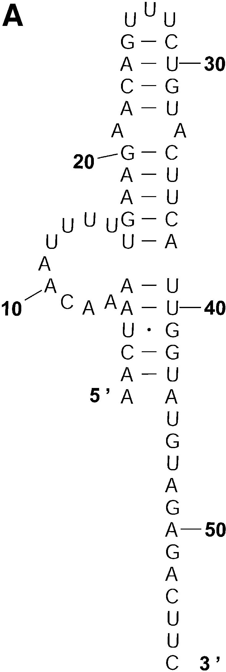
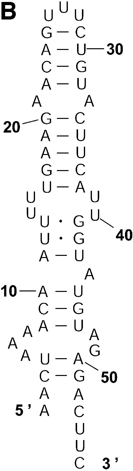
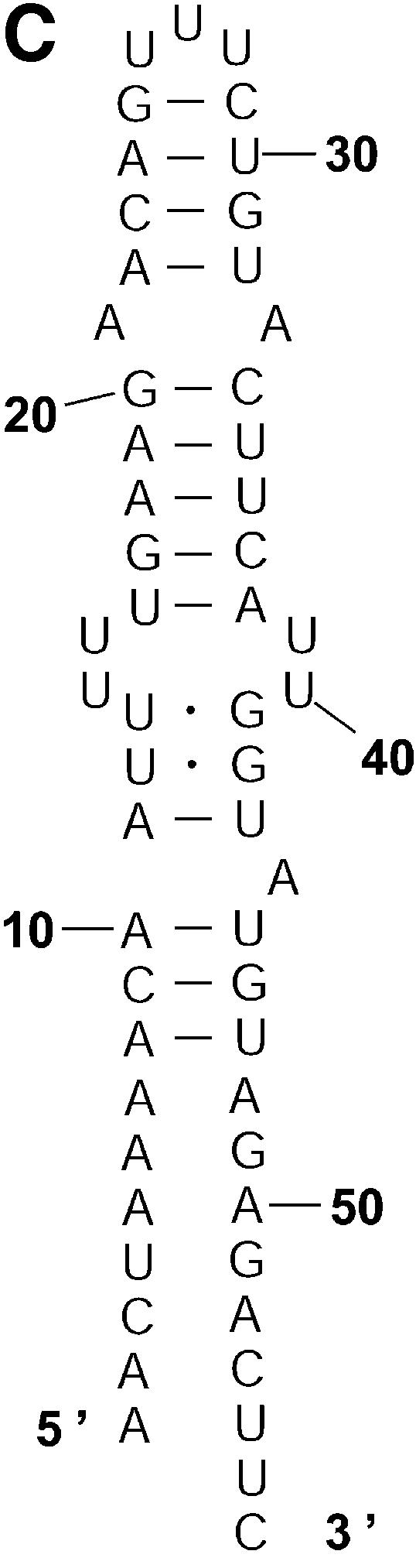
The representative structures for classes 1A, 1B and 1C for L.collosoma SL RNA. (A) Structure form 1 (20) for class 1A. (B) The optimal folding by mfold for class 1B. (C) The representative for class 1C.
Figure 5.

The representative structures for classes 2A and 2B for L.collosoma SL RNA. (A) Structure form 2 (20) for class 2A. (B) The representative for class 2B.
Figure 6.

Bar plot comparing the probability (estimated by the frequency in a sample) of a class (open bar) with the Boltzmann probability (filled bar) for the representative structure of a class. Classes are from the structure classification for L.collosoma SL RNA.
Entropic class. For class 2B, the ratio of the class probability to the Boltzmann probability of its most probable member is 290.70, which is strikingly high. Despite the very small Boltzmann probability for its most probable member, this group contains a substantial number of similar structures such that the collection of these structures has a much higher aggregate probability than the probability of each group member. Such ‘entropic classes’ of structures can be revealed by sampling and classification of sampled structures. However, a structure in an entropic class can be easily overlooked, when it is examined individually on the basis of its free energy or Boltzmann probability.
Table 3 presents a summary of the above analyses. Although the two experimental structures are 25.2% and 15.9% away from the MFE, respectively, they are both predicted by the sample. This sequence was also folded on the mfold server. For suboptimality percentage P under 15 (default = 5), only the optimal folding is returned. For a large P, e.g. P = 30, the two alternative structures are returned, among three suboptimal foldings. This example underscores the importance of examining suboptimal structures. It also shows that important alternative structures and structural motifs can be revealed by a statistical sample of the Boltzmann ensemble. These findings suggest that the Boltzmann ensemble of secondary structures for an RNA molecule can be adequately represented by the classes determined in a sample and the probabilities of the classes, together with the class-representative structures and their Boltzmann probabilities.
Table 3. Classification, representation and statistical characterization of the Boltzmann ensemble of the secondary structures for L.collosoma SL RNA, through the examination of a statistical sample of 1000 secondary structuresa.
| Class (2Dhist) | Probability | Representative structure | ΔG°37 (kcal/mol) (% away from MFE) | Boltzmann probability | Probability ration |
|---|---|---|---|---|---|
| 1A (Fig. 2A) | 0.010 | Fig. 4A (form 1) | –8 (25.2%) | 0.003598 | 2.78 |
| 1B (Fig. 2B) | 0.417 | Fig. 4B | –10.7 (0%) | 0.287469 | 1.45 |
| 1C (Fig. 2C) | 0.473 | Fig. 4C | –10.1 (5.6%) | 0.108593 | 4.36 |
| 2A (Fig. 3A) | 0.073 | Fig. 5A (form 2) | –9 (15.9%) | 0.018226 | 4.01 |
| 2B (Fig. 3B) | 0.025 | Fig. 5B | –5.7 (65.5%) | 0.000086 | 290.70 |
Prediction of alternative structures
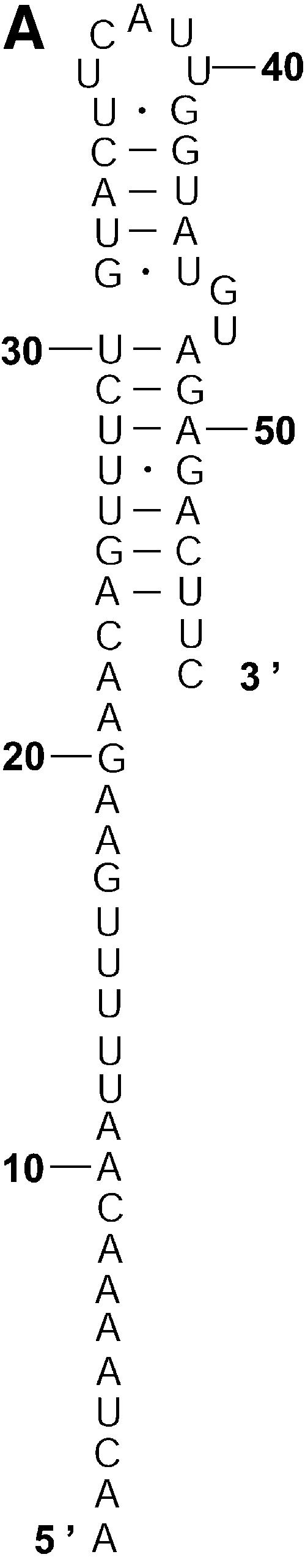
The analysis of L.collosoma SL RNA suggests that alternative biological structures can be adequately revealed by a statistical sample. We investigate this further by applying the sampling algorithm to prediction of mRNA secondary structures. mRNA secondary structures can play a regulatory role in determining the rate of translation initiation (9). This is explained by a model of co-existing alternative structures: one structure favors the translation initiation while the other inhibits the translation initiation (9). Also, it has been argued that the accessibility of the initiation codon is important for maximization of expression (22). The secondary structure of an mRNA is generally unavailable from experimental methods, because complete structural probing by chemical or enzymatic methods is very difficult for long-chain RNAs. A rare exception is the short mRNA for the cIII gene of bacteriophage λ, for which two conformations A and B (Fig. 7A and B) were elucidated and were demonstrated to co-exist in equilibrium (8). The sequence of 132 nt in the structures spans 46 nt of the coding region and 86 nt upstream from the initiation codon _A_0_UG_2. In structure A, the initiation codon and part of the Shine–Dalgarno sequence _U_–13_AAGGAG_–7 are in a closed, base-paired conformation such that the ribosome-binding site is occluded. In structure B, the ribosome-binding site is accessible for interactions. It is speculated that the cIII gene expression is regulated at the level of translation initiation through the ratio of the two structures at equilibrium, and through changes in temperature or Mg2+ concentration; perhaps ribosome binding can also shift the equilibrium (8). For the mRNA sequence of the cIII gene, a sample of 100 structures was generated by our algorithm and was manually examined. In this sample, 89 are close variants of structure A. The left-most stem in structure A is precisely predicted in 67 of the 89 structures. The exact right-most stem or a modification with one or both of additional pairs _A_–12–_U_42, _A_–11–_U_41 is predicted in 72 of the 89 structures. Appreciable variability in the location of the interior and bulge loops is observed for the middle stem. Structure C in Figure 7C is one of three structures in the sample that closely resemble structure B. The appreciable modification is the additional short helix involving the Shine–Dalgarno sequence formed by base pairs _G_–10·_C_44 and _G_–9·_C_43. The remaining eight structures (structures not shown) in the sample do not resemble either structure A or B, and have diverse structural features. The optimal folding by mfold is a modification of structure A with three additional base pairs _C_–54·_G_–35, _A_–12–_U_42 and _A_–11–_U_4, with an MFE of Δ_G_°37 = – 48.5 kcal/mol. Structure A is well predicted by the optimal folding. Its free energy is Δ_G_°37 = – 46.1 kcal/mol, 5% away from the MFE. Structure B has Δ_G_°37 = – 40.2 kcal/mol, 17% away from the MFE. Structure C has Δ_G_°37 = – 42.9 kcal/mol, 12% away from the MFE. For P = 30, neither B nor a variant resembling B as closely as C is predicted by suboptimal foldings from mfold, although both structures B and C are well within this range of suboptimality. By using the option for specifying base pair constraint in mfold, we verified that structures B and C are indeed present in the ‘missing’ set of suboptimal foldings that are excluded by the algorithm design for mfold, as discussed in the Introduction. In contrast to the stability indicated by the free energies, experimental analysis showed that structure B is favored by a factor of ∼3 (8). The discrepancy could be explained by tertiary interactions that preferentially stabilize structure B (8). This application not only exemplifies that an important alternative structure can be better predicted by a sample of moderate size, but it also shows that alternative structures of low probability can be biologically important, because stability contributions from potential tertiary interactions are unaccounted for. The finding also suggests that the sampling algorithm is well suited to the prediction of secondary structure of mRNAs, because an mRNA may exist as a population of conformations in an intracellular environment (5).
Figure 7.


Alternative structures for the mRNA of the cIII gene of bacteriophage λ. The initiation codon and the Shine–Dalgarno sequence are _A_0_UG_2 and _U_–13_AAGGAG_–7. The substructure from the 5′ end to nucleotide _A_–9 is the same for structure A and structure B. (A) Structure A proposed by Altuvia et al. (8). (B) Structure B proposed by Altuvia et al. (8). (C) Structure C represents a modification of B by an additional short helix involving a part of the Shine–Dalgarno sequence.
Assignment of probabilities to structural motifs
In many applications, certain types of structural motifs are of biological interest. Sampling also enables probabilistic prediction of any motif, with or without specific constraint(s). The probability of a motif can be directly estimated by the frequency of that motif’s occurrence in a sample. For the mRNA of the cIII gene of bacteriophage λ, this is illustrated in Table 4 for several constrained motifs involving the AUG initiation codon or the Shine–Dalgarno sequence, and for a helix, a base pair and a single-stranded fragment of two bases.
Table 4. Probability estimates of structural motifs for the mRNA of the cIII gene of bacteriophage λ from a sample of 100 structures.
| Motif and constraint | Probability |
|---|---|
| AUG initiation codon in a closed region (Fig. 7A) | 0.95 |
| AUG initiation codon in a partly open region (Fig. 7B and C) | 0.05 |
| At least four bases in either end of the Shine–Dalgarno sequence are in a helical region (Fig. 7A) | 0.97 |
| The ends of the Shine–Dalgarno sequence are open, but the bases in the middle are in a short helix (Fig. 7C) | 0.03 |
| The first helix from the 5′ end with 8 bp | 0.69 |
| Base pair _U_13–_G_20 | 0.93 |
| Unpaired _C_–40 and _U_–39 (in a hairpin) | 1.0 |
Probability profiling for predicting accessible regions in RNA secondary structure
Single-stranded regions in RNA secondary structure may be accessible for RNA:DNA, RNA:RNA and RNA:protein interactions. For prediction of accessible sites for targeting by antisense oligonucleotides, we developed a probability profiling approach based on the sampling algorithm (23). On a profile for fragment width W, the probability that W consecutive bases are all unpaired is plotted against the first base of the segment. This approach was shown to make substantially better predictions than the MFE structure. The significance of assigning probability as a measure of confidence in prediction is also highlighted by Figure 8A: a single-stranded region (nucleotides 26–37) predicted by both the MFE structure and the ss-count statistic from mfold has low probabilities on the probability profile [_W_ = 4 bases, as described in Ding and Lawrence (23)]. The ss-count statistic gives the propensity of a base to be unpaired, as measured by the frequency with which it is unpaired in a group of the optimal and suboptimal foldings within a specified increment of the MFE. For this RNA sequence, the same ss-count values were returned for suboptimality percentages P = 5 and P = 30. These values were averaged for W = 4 bases and were converted to the probability scale. Figure 8B illustrates a case of several substantial probability peaks on the profile (W = 4 bases), with little signal from the MFE structure, but more comparable predictions by ss-count. These cases occur when the MFE structure and the majority of the competing structures do not have a similar local structure. For the entire 1346 nt sequence, the correlation between ss-count and the profile probability is 0.6592 for W = 4. This correlation decreases to 0.5482 for W = 10. The MFE structure has commonly been used by experimentalists for antisense nucleic acid design, although with limited success (24). It is thus important to consider suboptimal foldings in the selection of antisense target sites. The probability profiling approach has the advantage that it fully assesses the uncertainty in the predictions.
Figure 8.


Comparison of predictions by sampling and by free energy minimization. At nucleotide position i, the probability that nucleotide i, i + 1, i + 2, i + 3 (i.e. fragment width W = 4) are all single stranded is plotted against i. This probability is computed by a sample of 1000 structures (probability profile), by MFE structure and by ss-count from mfold for the nucleotides 1–60 (A) and 1262–1322 regions (B) of the mRNA for H.sapiens γ-glutamyl hydrolase (GenBank accession No. U55206, with 66 additional nucleotides at the 5′ end).
Probability profiling for specific loop types
A probability profile statistically delineates unpaired bases (W = 1) or fragments (W >1), regardless of the type of loop in which the base or fragment occurs. An extension to account for loop type is straightforward by keeping track of the loop type for unpaired bases returned from the sampling step. Thus, the sampling algorithm also enables probability profiling of a specific loop type.
For Escherichia coli tRNAAla, Figure 9 shows the profile plots (W = 1) Hplot, Bplot, Iplot, Mplot and Extplot, for hairpin loop, bulge loop, interior (internal) loop, multibranched loop and the exterior loop, respectively. For example, at sequence position i, Hplot presents the probability that nucleotide i is in a hairpin loop. The probability is computed by the observed frequency in a sample of 1000 structures. The three high probability regions on Hplot correspond to the regions for the D loop (_A_14_GCUGGGA_21), the anticodon loop (_A_32_UGGCAU_38) and the T_Ψ_C loop (_U_54UCGAUC60) in the cloverleaf conformation determined phylogenetically for this tRNA. There is no bulge or interior loop in the cloverleaf structure. Accordingly, there is little signal on Bplot, and only weak signal on Iplot. The three high probability regions on Mplot correspond to the three segments of unpaired bases (_U_8_A_9, _G_26 and _A_44_GGUC_48) in the multibranched loop of the cloverleaf. The high probability segment on Extplot corresponds to the four free dangling bases (_A_73_CCA_76) on the 3′ end of the cloverleaf structure. Interestingly, Extplot indicates that ∼16% of the sampled structures have _A_14_GC_16 as the junction that connects two separate folding domains.
Figure 9.


Loop profiles for E.coli tRNAAla. (A) Hplot displays the probability that a base lies in a hairpin loop; (B) Bplot displays the probability that a base is in a bulge loop; (C) Iplot displays the probability that a base is in an interior (internal) loop; (D) Mplot displays the probability that a base is in a multibranched loop; and (E) Extplot displays the probability that a base is in the exterior loop.
The most intriguing observation is that not only is the anticodon loop (second peak from the left in Hplot) the most conserved among three hairpin loops, but it also is the most conserved accessible region for any loop type. The respective probabilities on Hplot for the three anticodon bases _G_34, _G_35 and _C_36 are 0.968, 0.961 and 0.962. Thus, possible alternative foldings of this tRNA in the intracellular environment are highly unlikely to affect the accessibility of the anticodon for base pairing with the codon on the mRNA. In other words, for this tRNA, the function of codon recognition is preserved with high certainty even if the folding deviates from the classic cloverleaf. Further analysis of other tRNA sequences from the tRNA database (2) is warranted to assess the degree of generality of such predicted anticodon accessibility. Before such an analysis, an extension of the algorithm for partition functions needs to be developed to allow constraints, because many tRNAs have modified bases that cannot be involved in base pairing.
Mutual accessibility plot for prediction of RNA:RNA interaction
For RNA:RNA interactions through antisense binding, e.g. between an RNA target and chemically synthesized or natural occurring antisense RNAs, or between an RNA target and _trans_-cleaving ribozymes, the structures of both RNAs are important. Antisense binding is largely dependent on the accessibility of both the bases at the target site and the complementary bases on the antisense RNA or ribozyme. This mutual accessibility between two RNAs can be assessed with an overlay plot of probability profiles for the two RNAs at the target site (Fig. 10).
Figure 10.


(A) Mutual accessibility plot obtained by overlaying probability profiles (fragment width W = 4) at the target site for a 60 nt antisense RNA (embedded in a long RNA through an expression vector) and the targeted mRNA of H.sapiens γ-glutamyl hydrolase. Both the RNA containing the 60 nt antisense insert and the entire target mRNA were folded. Fairly good mutual accessibility is predicted by the overlapping high probability region between nucleotides 730 and 750. (B) For the mRNA of H.sapiens breast cancer resistance protein (BCRP; GenBank accession No. AF098951) and an hammerhead ribozyme designed for a GUC cleavage sequence on the target, fairly good mutual accessibility for the nucleation step of antisense binding is predicted for both the target and the two binding arms of the ribozyme (W = 1 for the probability profiles).
The mutual accessibility plot provides a new tool to address local accessibility of both RNAs at the target site, in addition to the uncertainty in the RNA folding predictions. This tool can be valuable for the rational design of ribozymes and antisense RNAs for gene inhibition. Based on the mutual accessibility plot, we have tested three hammerhead ribozymes against breast cancer resistance protein (BCRP) in cultured cells. All three ribozymes were successful in substantially reducing the levels of the protein (K.Kowaski, Y.Ding and E.Schneider, unpublished data).
Boltzmann probability-weighted density of states and free energy distributions
Cupal and co-workers (25) presented a recursive algorithm to compute the free energy distribution of all secondary structures (i.e. the density of states, or DOS). The algorithm is O(_n_5) in time with a memory requirement of O(_n_3), and is thus computationally prohibitive even for sequences of moderate length. For short sequences, this algorithm is useful for the study of evolution, through comparison of DOS between biological sequences and random sequences of the same composition (26).
A sampling estimate of the free energy distribution of probable structures is readily available from our sampling algorithm and is referred to as the Boltzmann probability-weighted density of states, or BPWDOS (Fig. 11A), because structures are sampled with Boltzmann equilibrium probabilities. Information for the BPWDOS can be displayed in alternative forms for depiction of the probability that a structure lies within a threshold of the MFE, or in a free energy interval (Fig. 11B and C). For a specified low energy interval, sampling also generates representative structures for further examination. This overcomes the disadvantage of the algorithm by Cupal and co-workers that no information exists about individual structures corresponding to the low energy states. Such distributions could be valuable in evolutionary studies on long sequences and studies of the RNA energy landscape (27). Similarly, other sampling statistics, such as the distribution of the number of base pairs in sampled structures, can be computed.
Figure 11.


For L.collosoma SL RNA, (A) Boltzmann probability-weighted density of states (BPWDOS); (B) probability of a structure having a free energy within P% of the minimum free energy; (C) probability of a structure having a free energy within a specified _P_-interval.
Sample size and statistical reproducibility
The calculation of sampling statistics is typically based on a sample of 1000 structures. To assess the adequacy of this sample size, we generated two independent samples for the mRNA of _Homo sapiens N_-acetylglucosamine kinase, 1187 nt in length. Each sample contains 1000 structures. For this sequence, an estimate of the number of all secondary structures is 1.81187 ≈ 10303. From the 2Dhist, the patterns of base pair frequencies are nearly identical for the two samples (Fig. 12A, first sample; Fig. 12B, second sample). The probability profiles (W = 4) for both samples are also computed and are overlaid in a single plot, by plotting against common nucleotide position (Fig. 13A). The two profile curves are colored red and blue, respectively. However, the overlay plot is overwhelmingly dominated by the blue color; the red curve is hardly visible when the two profiles overlap. The red curve is observed only in the case of distinguishable variation. This statistical phenomenon is better observed by an enlargement of a 200 nt region shown in Figure 13B.
Figure 12.


Statistical reproducibility is illustrated by 2Dhist for two independent samples of 1000 structures each for the mRNA of _H.sapiens N_-acetylglucosamine kinase. The histograms (A and B) display nearly identical patterns of base pair probabilities estimated by sampling.
Figure 13.


Statistical reproducibility is illustrated by nearly complete overlapping of probability profiles for two independent samples of 1000 structures each for the mRNA of _H.sapiens N_-acetylglucosamine kinase. (A) Complete profiles for the entire mRNA. (B) An enlargement of the profile for the nucleotide 400–600 region.
Furthermore, through a pairwise structural comparison, we found that the two samples do not have a single structure in common. Thus, it might initially appear to be surprising that, for an ensemble of ∼10303 structures, a sample of only 1000 structures can yield statistical reproducibility of typical sampling statistics, even if samples can be entirely different. However, these results are fully expected, because a sample generated by the algorithm is guaranteed to be statistically representative. A simple analogy is sampling from the US population of 280 million persons. If two random samples of individuals are taken independently with a sample size of 1000, it is highly likely that the two samples will not have a single individual in common, because the population is large, and because sampling is not only random but also independent. However, the two samples would produce highly consistent estimates for demographic characteristics, such as the percentage of males in the population.
Although the precision in the estimates of sampling statistics does increase with sample size, a sample size of 1000 structures is adequate for most applications. Nevertheless, in the case that a rare event of small Boltzmann probability is of interest, the sample size can be increased to improve the precision in the estimates. For example, for the L.collosoma SL RNA, a sample size of 1 000 000 structures is used, because the Boltzmann probability for experimental structure 1 is merely 0.0036 (Table 1).
Availability of software _S_fold
Based on the structure sampling algorithm and the novel tools, we have developed a software packaged named _S_fold, for statistical RNA folding and rational design of RNA-targeting nucleic acids. _S_fold is available through Web servers at http://sfold.wadsworth.org and http://www.bioinfo.rpi.edu/applications/sfold.
DISCUSSION
We have presented a novel statistical algorithm to sample RNA secondary structures exactly and rigorously, according to the Boltzmann equilibrium probability distribution of the secondary structures for a given RNA sequence. The forward step of the algorithm for calculating partitions functions is cubic when long interior loops are prohibited, and the backward sampling step can rapidly generate a large, statistically representative sample of structures. A sample generated by the algorithm is guaranteed to be statistically representative. Characteristics of the Boltzmann ensemble revealed by sampling are statistically reproducible for independent samples of moderate size.
In the full ensemble of secondary structures for an RNA sequence, some structures are very similar, while others are substantially different. Although it is not computationally feasible to enumerate and classify all structures, the results on L.collosoma SL RNA show that the ensemble can be partitioned into mutually exclusive classes. Like the individual structures, the classes are not equally probable. The structure sample size of 1000 used in our classification analysis sets a probability threshold of 0.001. Classes with Boltzmann probabilities that are significant relative to the threshold are expected to be represented in the sample. Classes with insignificant probabilities are unlikely to be observed in the sample. Thus, sampling provides an efficient means to statistically delineate the Boltzmann ensemble of secondary structures through significant classes. The development of an algorithm for the determination of distinct classes will thus be an important topic of future research.
The sampling algorithm enables a rigorous statistical description of uncertainties in RNA folding prediction. The demonstrated new predictive insights and novel application tools are unique to this algorithm. The sampling approach avoids the limitation of suboptimal folding presentation by a designed set. It also bypasses the difficulty associated with a complete enumeration and examination of all suboptimal foldings within a specified increment of the MFE.
Prediction of suboptimal foldings is important, because the biological structures may not be well predicted by the MFE structure. Even for RNAs with possibly unique structures, the sampling approach has the advantage of addressing uncertainty in the predictions.
The algorithm is shown to meet the challenges of predicting alternative biological structures and of making an adequate representation of suboptimal foldings. The improved predictions in applications to mRNAs reported both here and in our previous work suggest that the sampling algorithm and the probability profile approach are well suited to the prediction of mRNA secondary structures and to the assessment of target accessibility, because an mRNA may exist as a population of different structures, and a stochastic approach to accessibility evaluation may be appropriate (5). The probability profiling approach reveals target sites that are commonly accessible for a large number of statistically representative structures for the target RNA. Through rigorous assignment of statistical confidence in predictions, this novel approach bypasses the long-standing difficulty of how to select a single structure for accessibility evaluation.
For antisense oligonucleotides and _trans_-cleaving ribozymes, it has been well established that the target accessibility is primarily determined by the secondary structure of the target RNA. Recently, experimental evidence has emerged to support the idea that the potency of small interfering RNAs (siRNAs) is also determined by the target secondary structure and accessibility (28–31). In the post-genomic era, reverse genetic tools based on these RNA-targeting nucleic acids are becoming increasingly important for high throughput functional genomics, drug target validation and development of human therapeutics. The probability profiling method and the mutual accessibility plot are useful tools for the rational design of RNA-targeting nucleic acids for gene knock-down studies, as well as for the design of nucleic acid probes such as molecular beacons for tracing mRNAs (32). Based on probability profiling, we have designed antisense oligonucleotides against E.coli lacZ, and siRNAs against the human estrogen receptor. Results from preliminary testing in cell extracts and in cultured cells are highly encouraging (a summary of our unpublished data is available on the _S_fold Web sites). Large-scale experimental testing is warranted to further validate the novel design methodology.
Acknowledgments
ACKNOWLEDGEMENTS
We thank D.H. Mathews and D.H. Turner for making free energy parameters available to us and for interpretation of the parameters, and D.H. Mathews for a suggestion that significantly improved the run time for the calculation of partition functions. We also thank K. McDonough, E. Schneider, B. Pentecost, and M. Fasco for preliminary testing of antisense oligonucleotides, hammerhead ribozymes and siRNAs. The Computational Molecular Biology and Statistics Core at the Wadsworth Center is acknowledged for providing computing resources for this work. The secondary structure displays in Figures 4, 5 and 7 were produced using the XRNA interactive program (http://rna.ucsc.edu/rnacenter/) developed by Bryn Weiser and Harry Noller at the University of California, Santa Cruz. The two-dimensional histograms for Figures 2 and 3 were generated by Histo-Scope and NPlot, an interactive histogramming and plotting program (http://www.fnal.gov/fermitools/abstracts/histoscope/abstract.html) developed by George Dimas and Mark Edel at Fermi National Accelerator Laboratory, Batavia, Illinois. The long-term development of the _S_fold software is supported by National Science Foundation grant DMS-0200970 and National Institutes of Health grant GM068726 to Y.D. Chiyu Chan is responsible for the development of the graphical tools and the Web user interface.
APPENDIX: RECURSIONS FOR EQUILIBRIUM PARTITION FUNCTIONS
The structural elements in RNA secondary structure include helix, hairpin loop, bulge loop, interior (internal) loop and multibranched loop (Fig. A1). The exterior loop consists of free dangling bases on the 5′ end and the 3′ end, and bases in the junction between two separate folding domains.
When an unpaired base is adjacent to two helices, we only consider the 3′ dangling, because it is usually more energetically favorable than 5′ dangling, according to the free energy data for dangling ends (33). The assumed additivity of free energy implies multiplicativity of contributions by structural elements to the partition functions. The contributions to the partition functions by mutually exclusive conformational cases are, however, additive. These features are important in the derivation of a recursive algorithm for partition functions.
Recursions
For fragment R_ij_, it can be either single stranded or there is at least one base pair on the fragment. In the latter case, if we consider the base pair r h –r l closest to the 5′ end of the fragment [the first (h_–_i) bases are thus single stranded], we then have the following mutually exclusive and exhaustive cases, as illustrated by Figure A2: (a) R ij is single stranded; (b) h = i, l = j; (c) i < h < l = j; (d) h = i < l < j; (e) i < h < l < j. Thus, u(i, j) is a sum of five terms:
u(i, j) = 1 + up(i, j)exp[– etp(i, j)/RT_] + Σ_i < h < j up(h, j)exp{– [ed_5(h, j, h – 1) + etp(h, j)]/RT} + Σ_i < l < j up(i, l)exp[– etp(i, l)/RT]{exp[– _ed_3(i, l, l + l)/RT_]u(l + 2, j) + u(l + 1, j) – u(l + 2, j)} + Σ_i < h < l < j up(h, l)exp{– [_ed_5(h, l, h – 1) + etp(h, l)]/RT}{exp[– _ed_3(h, l, l + 1)/RT]u(l + 2, j) + u(l + 1, j) – u(l + 2, j)} A1
where for base pair r i –r j, etp(i, j) is the terminal A_–_U, G_–_U penalty, and ed_5(h, l, h – 1) is the free energy for 5′ dangling r h – 1 on r h –_r l, and ed_3(h, l, l + 1) is the free energy for 3′ dangling r l + 1 on r h –_r l. When r i and r j form a base pair, there are the following exclusive and exhaustive cases: (i) r i –r j closes a hairpin; (ii) r i –r j is the exterior pair of a base pair stack; (iii) r i –r j closes a bulge or an interior loop; or (iv) r i –r j closes a multibranched loop. Thus, up(i, j) is the sum of four contributions:
up(i, j) = exp[–eh(i, j)/RT_] + exp[–_es(i, j, i + 1_, j_ – 1)/RT]up(i + 1, j – 1) + Σ_i < h < l < j_ exp[–ebi(i, j, h, l)/_RT_]up(h, l) + up m (i, j) A2
where eh(i, j), es(i,j, i + l, j – 1) and ebi(i, j, h, l) are, respectively, the free energies for a hairpin closed by r i –r j, for stacking between base pairs r i –r j and r i + 1 –r j – 1, and for a bulge or an interior loop with exterior base pair r i –r j and interior base pair r h –r l, while up m (i, j) is the contribution from case (iv). For case (iv), if we consider the internal helix closest to r i with closing pair r h –r l, the recursion for up m (i, j) is
up m (i, j) = Σ_i_ + 1 < l < j up(i + 1, l)exp{–[a + 2_c_ + etp(i + 1, l)]/RT}{exp[–_ed_3(i + 1, l, l + 1)/RT_]u_1(l + 2, j – 1) + u_1(l + 1, j – 1) – u_1(l + 2, j – 1)} + Σ_i + 2 < l < j up(i + 2, l)exp{–[a + 2_c + b + _ed_3(j, i, i + 1) + etp(i + 2, l)]/RT}{exp[–_ed_3(i + 2, l, l + 1)/_RT_]_u_1(l + 2, j – 1) + u_1(l + 1, j – 1) – u_1(l + 2, j – 1)} + Σ_i + 3 ≤ h < l < j up(h, l)exp{–[a + 2_c + (h – i – 1)b + _ed_3(j, i, i + 1) + _ed_5(h, l, h – 1) + etp(h, l)]/RT}{exp[–_ed_3(h, l, l + 1)/_RT_]_u_1(l + 2, j – 1) + _u_1(l + 1, j – 1) – _u_1(l + 2, j – 1)} A3
where a, b, c are the offset, free base penalty and helix penalty of the assumed linear penalty for a multibranched loop: loop penalty = a + b(number of unpaired bases) + c(number of helices); the three sums with h = i + l, h = i + 2 and h ≥ i + 3 are for different cases of dangling on r i –r j and r h –r l. u_1(k, j – 1) is an auxiliary partition function for a multibranched loop with the following properties: there is at least one helix between r k and r j – 1 ; r k – 1 is the 3′ end of the previous helix in the loop; r j is the 3′ end base of the closing pair r i –_r j for the loop. Similar to the derivation of up m (i, j), we consider the closing base pair r h ′ –r l ′ of the helix closest to the 5′ end of R( l + 1) j, and we take into account both the dangling energy and the terminal penalty. Furthermore, we must consider both the case of no additional helix between r l ′ + 1 and r j and the case of at least one more helix. For _u_1(i, j), r j + 1 is the 3′ base of the closing base pair for the multibranched loop, and r i – 1 is the 3′ end of the previous helix in the loop. The recursion for _u_1(i, j) is:
u_1(i, j) = Σ_i < l ≤ j up(i, l)exp{–[c + etp(i, l)]/RT}{f(j + 1, i, l)exp[–(j – l)b/_RT_] + exp[–_ed_3(i, l, l + 1)/_RT_]u_1(l + 2, j) + u_1(l + 1, j) – u_1(l + 2, j)} + Σ_i + 1 < l ≤ j up(i + 1, l)exp{–[c + b + etp(i + 1, l)]/RT}{f(j + 1, i + 1, l)exp[–(j – l)b/_RT_] + exp[–_ed_3(i + 1, l, l + 1)/_RT_]_u_1(l + 2, j) + _u_1(l + 1, j) – u_1(l + 2,j)} + Σ_i + 2 ≤ h < l ≤ j up(h, l)exp{–[c + (h – i)b + etp(h, l) + _ed_5(h, l, h – 1)]/RT}{f(j + 1, h, l)exp[–(j – l)b/_RT_] + exp[–_ed_3(h, l, l + 1)/_RT_]_u_1(l + 2, j) + _u_1(l + 1, j) – _u_1(l + 2, j)} A4
where f(j + l, h, l) = 1 for l = j and f(j + l, h, l) = exp[–_ed_3(h, l, l + 1)/_RT_] for l < j. The computation is O(_n_4) for equations A1, A3 and A4 as written, and it is O(_n_3) for equation A2 when long interior loops are disallowed. We introduce three additional auxiliary arrays _s_1(h, j), _s_2(h, j) and _s_3(h, j):
s_1(h, j) = Σ_h < l < j up(h, l)exp{–[_ed_5(h, l, h – 1) + etp(h, l)]/RT}{exp[–_ed_3(h, l, l + 1)/_RT_]u(l + 2, j) + u(l + 1, j) – u(l + 2, j)} A5
s_2(h, j) = Σ_h < l < j up(h, l)exp{–[_ed_5(h, l, h – 1) + etp(h, l)]/RT}{exp[–_ed_3(h, l, l + 1)/_RT_]_u_1(l + 2, j – 1) + _u_1(l + 1, j – 1) – _u_1(l + 2, j – 1)} A6
s_3(h, j) = Σ_h < l ≤ j up(h, l)exp{–[_ed_5(h, l, _h_-1) + etp(h, l)]/RT}{f(j + 1, h, l)exp[–(j – l)b/_RT_] + exp[–_ed_3(h, l, l + 1)/_RT_]_u_1(l + 2, j) + _u_1(l + 1, j) – _u_1(l + 2, j)} A7
Then, the quartic sum in equation A1 becomes Σ_i_ < _h_ < _j_ – 1 _s_1(_h_, _j_), the quartic sum in equation **A3** becomes exp[(–_ed_3(_j_, _i_, _i_ + l)/_RT_] Σ_i_ + 3 ≤ _h_ < _j_ – 1 exp [–(_a_ + 2_c_ + (_h_ – _i_ – 1)_b_)/ _RT_]_s_2(_h_, _j_), and the quartic sum in equation **A4** becomes Σ_i_ + 2 ≤ _h_ ≤ _j_ – 1 exp [–(_c_ + (_h_ – _i_) _b_)/_RT_ ]_s_3(_h_, _j_). At the cost of storage of these arrays, the algorithm is cubic when long interior loops (e.g. size >30) are disregarded.
Boundary values
We start the computation with boundary values for short fragments and proceed to longer ones using the recursions. For 1 ≤ i ≤ j ≤ i + 3 ≤ n, u(i, j) = 1, up(i, j) = 0, _u_1(i, j) = 0, _s_1(i, j) = 0, _s_2(i, j) = 0, and _s_3(i, j) = 0; for j = i + 4 ≤ n, u(i, i + 4) = 1 + exp[–(_eh_(3) + etp(i, i + 4))/_RT_], up(i, i + 4) = exp[–_eh_(3)/_RT_], _u_1(i, i + 4) = exp[–(_c_ + _eh_(3) + etp(i, i + 4))/_RT_], _s_1(i, i + 4) = 0, _s_2(i, i + 4) = 0, and _s_3(i, i + 4) = exp[–(_eh_(3) + etp(i, i + 4) + _ed_5(i, i + 4, i – 1 )/_RT_]; for 1 ≤ i ≤ n, u(i + l, i) = 1, _u_1(i + l, i) = 0; and for 1 ≤ i ≤ n – 1, _u_1(i + 2, i) = 0.
Figures
Figure a1.

Elements of RNA secondary structure: helix, hairpin loop, bulge loop, interior (internal) loop and multibranched loop.
Figures
Figure a2.

In the derivation of recursions for u(i, j), mutually exclusive and exhaustive cases are enumerated by considering fragment R ij being single stranded or the base pair r h –r l closest to the 5′ end of the fragment [i.e. the first (h_–_i) bases are single stranded]: (a) R ij is single stranded; (b) h = i, l = j; (c) i < h < l = j; (d) h = i < l < j; and (e) i < h < l < j.
REFERENCES
- 1.More P.B. and Steitz,T.A. (2003). The structural basis of large ribosomal subunit function. Annu. Rev. Biochem., 72, 813–850. [DOI] [PubMed] [Google Scholar]
- 2.Sprinzl M., Horn,C., Brown,M., Ioudovitch,A. and Steinberg,S. (1998) Compilation of tRNA sequences and sequences of tRNA genes. Nucleic Acids Res., 26, 148–153. [DOI] [PMC free article] [PubMed] [Google Scholar]
- 3.McCaskill J.S. (1990) The equilibrium partition function and base pair binding probabilities for RNA secondary structure. Biopolymers, 29, 1105–1119. [DOI] [PubMed] [Google Scholar]
- 4.Bonhoeffer S., McCaskill,J.S., Stadler,P.F. and Schuster,P. (1993) RNA multi-structure landscapes. A study based on temperature dependent partition functions. Eur. Biophys. J., 22, 13–24. [DOI] [PubMed] [Google Scholar]
- 5.Christoffersen R.E., McSwiggen,J.A. and Konings,D. (1994) Application of computational technologies to ribozyme biotechnology products. J. Mol. Struct. (Theochem.), 311, 273–284. [Google Scholar]
- 6.Weidner H., Yuan,R. and Crothers,D.M. (1977) Does 5S RNA function by a switch between two secondary structures? Nature, 266, 193–194. [DOI] [PubMed] [Google Scholar]
- 7.Jagadeeswaran P. and Cherayil,J.D. (1980) A general model for the conformational switch in 5S RNA during protein synthesis. J. Theor. Biol., 83, 369–375. [DOI] [PubMed] [Google Scholar]
- 8.Altuvia S., Kornitzer,D., Teff,D. and Oppenheim,A.B. (1989) Alternative mRNA structures of the cIII gene of bacteriophage λ determine the rate of its translation initiation. J. Mol. Biol., 210, 265–280. [DOI] [PubMed] [Google Scholar]
- 9.Stormo G. (1986) Translation initiation. In Reznikoff,W. and Golg,L. (eds), Maximizing Gene Expression. Butterworth Publishers, Stoneham, MA, pp. 195–224. [Google Scholar]
- 10.Landick R., Turnbough,C.L. and Yanofsky,C. (1996) Transcription attentuation. In Neidhardt,F.C., Curtiss,R. and Lin,E.C (eds), Escherichia coli and Salmonella: Cellular and Molecular Biology, 2nd edn. American Society for Microbiology, Washington, DC, pp. 1263–1286. [Google Scholar]
- 11.Zuker M. (2000) Calculating nucleic acid secondary structure. Curr. Opin. Struct. Biol., 10, 303–310. [DOI] [PubMed] [Google Scholar]
- 12.Zuker M. and Stiegler,P. (1981) Optimal computer folding of large RNA sequences using thermodynamics and auxiliary information. Nucleic Acids Res., 9, 133–148. [DOI] [PMC free article] [PubMed] [Google Scholar]
- 13.Zuker M. (1989) On finding all suboptimal foldings of an RNA molecule. Science, 244, 48–52. [DOI] [PubMed] [Google Scholar]
- 14.Wuchty S., Fontana,W., Hofacker,I.L. and Schuster,P. (1999) Complete suboptimal folding of RNA and the stability of secondary structures. Biopolymers, 49, 145–165. [DOI] [PubMed] [Google Scholar]
- 15.Williams A.L. and Tinoco,I.,Jr (1986) A dynamic programming algorithm for finding alternative RNA secondary structures. Nucleic Acids Res., 14, 299–315. [DOI] [PMC free article] [PubMed] [Google Scholar]
- 16.Ding Y. and Lawrence,C.E. (1999) A Bayesian statistical algorithm for RNA secondary structure prediction. Comput. Chem., 23, 387–400. [DOI] [PubMed] [Google Scholar]
- 17.Ding Y. (2002) Rational statistical design of antisense oligonucleotides for high throughput functional genomics and drug target validation. Stat. Sin., 12, 273–296. [Google Scholar]
- 18.Xia T., SantaLucia,J.,Jr, Burkard,M.E., Kierzek,R., Schroeder,S.J., Jiao,X., Cox,C. and Turner,D.H. (1998) Thermodynamic parameters for an expanded nearest-neighbor model for formation of RNA duplexes with Watson–Crick base pairs. Biochemistry, 37, 14719–14735. [DOI] [PubMed] [Google Scholar]
- 19.Mathews D.H., Sabina,J., Zuker,M. and Turner,D.H. (1999) Expanded sequence dependence of thermodynamic parameters improves prediction of RNA secondary structure. J. Mol. Biol., 288, 911–940. [DOI] [PubMed] [Google Scholar]
- 20.LeCuyer K.A. and Crothers,D.M. (1993) The Leptomonas collosoma spliced leader RNA can switch between two alternate structural forms. Biochemistry, 32, 5301–5311. [DOI] [PubMed] [Google Scholar]
- 21.Fleiss J.L. (1981) Statistical Methods for Rates and Proportions, 2nd edn. John Wiley & Sons, New York. [Google Scholar]
- 22.Iserentant D. and Fiers,W. (1980) Secondary structure of mRNA and efficiency of translation initiation. Gene, 9, 1–12. [DOI] [PubMed] [Google Scholar]
- 23.Ding Y. and Lawrence,C.E. (2001) Statistical prediction of single-stranded regions in RNA secondary structure and application to predicting effective antisense target sites and beyond. Nucleic Acids Res., 29, 1034–1046. [DOI] [PMC free article] [PubMed] [Google Scholar]
- 24.Sohail M. and Southern,E.M. (2000) Selecting optimal antisense reagents. Adv. Drug Deliv. Rev., 44, 23–34. [DOI] [PubMed] [Google Scholar]
- 25.Cupal J., Flamm,C., Renner,A. and Stadler,P.F. (1997) Density of states, metastable states and saddle points exploring the energy landscape of an RNA molecule. Proceedings of ISMB97, pp. 88–91. [PubMed] [Google Scholar]
- 26.Higgs P.G. (1995) Thermodynamic properties of transfer RNA: a computational study. J. Chem. Soc. Faraday Trans., 91, 2531–2540. [Google Scholar]
- 27.Schuster P. and Stadler,P.F. (1994) Landscapes: complex optimization problems and biopolymer structures. Comput. Chem., 18, 295–324. [DOI] [PubMed] [Google Scholar]
- 28.Lee N.S., Dohjima,T., Bauer,G., Li,H., Li,M.J., Ehsani,A., Salvaterra,P. and Rossi,J. (2002) Expression of small interfering RNAs targeted against HIV-1 rev transcripts in human cells. Nat. Biotechnol., 20, 500–505. [DOI] [PubMed] [Google Scholar]
- 29.Vickers T.A., Koo,S., Bennett,C.F., Crooke,S.T., Dean,N.M. and Baker,B. (2003) Efficient reduction of target RNAs by small interfering RNA and RNase H-dependent antisense agents. A comparative analysis. J. Biol. Chem., 278, 7108–7118. [DOI] [PubMed] [Google Scholar]
- 30.Bohula E.A., Salisbury,A.J., Sohail,M., Playford,M.P., Riedemann,J., Southern,E.M. and Macaulay,V.M. (2003) The efficacy of small interfering RNAs targeted to the type 1 insulin-like growth factor receptor (IGF1R) is influenced by secondary structure in the IGF1R transcript. J. Biol. Chem., 278, 15991–15997. [DOI] [PubMed] [Google Scholar]
- 31.Far R.K. and Sczakiel,G. (2003) The activity of siRNA in mammalian cells is related to structural target accessibility: a comparison with antisense oligonucleotides. Nucleic Acids Res., 31, 4417–4424. [DOI] [PMC free article] [PubMed] [Google Scholar]
- 32.Tyagi S. and Kramer,F.R. (1996) Molecular beacons: probes that fluoresce upon hybridization. Nat. Biotechnol., 14, 303–308. [DOI] [PubMed] [Google Scholar]
- 33.Turner D.H., Sugimoto,N. and Freier,S.M. (1988) RNA structure prediction. Annu. Rev. Biophys. Biophys. Chem. 17, 167–192. [DOI] [PubMed] [Google Scholar]