Understanding the Evolution and Stability of the G-Matrix (original) (raw)
. Author manuscript; available in PMC: 2011 Dec 2.
Abstract
The G-matrix summarizes the inheritance of multiple, phenotypic traits. The stability and evolution of this matrix are important issues because they affect our ability to predict how the phenotypic traits evolve by selection and drift. Despite the centrality of these issues, comparative, experimental, and analytical approaches to understanding the stability and evolution of the G-matrix have met with limited success. Nevertheless, empirical studies often find that certain structural features of the matrix are remarkably constant, suggesting that persistent selection regimes or other factors promote stability. On the theoretical side, no one has been able to derive equations that would relate stability of the G-matrix to selection regimes, population size, migration, or to the details of genetic architecture. Recent simulation studies of evolving G-matrices offer solutions to some of these problems, as well as a deeper, synthetic understanding of both the G-matrix and adaptive radiations.
Keywords: Adaptive landscape, genetic variance-covariance matrix, phenotypic evolution, selection surface
The aim of this article is to review empirical, analytical, and simulation studies of the G-matrix with a focus on its stability and evolution. This review is timely because a series of emerging generalities about phenotypic evolution suggest that important methodological advances lie just around the comer. New insights into G-matrix evolution highlight certain themes in empirical work that in turn may lay the foundation for those advances.
The study of phenotypic evolution is at a crucial juncture as an onslaught of fresh empirical findings continues to foster the development of new methodological tools in comparative biology (Hohenlohe and Arnold 2008). On the empirical front, one can argue for five emerging generalizations, although controversy remains in some cases (Barton and Turelli 1989; Houle 1992; Barton and Keithley 2002; Marroig and Cheverud 2004; Blows and Hoffman 2005). (1) Genetic variation is abundant in most populations for many kinds of characters (Mousseau and Roff 1987). This apparent availability of genetic variation suggests that genetic constraints might play at most a minor or transitory role in adaptive radiation of simple traits such as size (Charlesworth et al. 1982; Estes and Arnold 2007). (2) A variety of lines of evidence suggest that phenotypic diversification is primarily driven by selection rather than by drift alone (Estes and Arnold 2007). (3) Significant evolutionary change can occur over a few generations, on an ecological timescale (Thompson 1998; Hairston et al. 2005). (4) Despite evident capacity for rapid evolutionary responses to environmental challenges, implied by (1–3), stasis is a prevalent–perhaps the most prevalent–mode of evolution, especially pronounced on long timescales (Gould 2002). (5) Correlated evolution of multiple traits is common, as reflected by consistent patterns of trait association that are apparent at all levels of divergence (Gould 1966; Harvey and Pagel 1991). Despite the prevalence of these evolutionary patterns, which are at the crux of adaptive radiation, we are still struggling to achieve a synthetic understanding of their causes. Thus, the challenge for the new analytical tools is to accommodate these emerging empirical generalizations, even as we continue to test them. An important conceptual realization is that our best hope of understanding correlated evolution and other patterns may lie with analytical tools that use two powerful multivariate concepts, the adaptive landscape and the G-matrix (Arnold et al. 2001). In other words, we argue that an understanding of the adaptive landscape and its effects on the G-matrix is central to a synthetic vision of emerging generalities in the field of phenotypic evolution. We begin with the adaptive landscape because it both directs the course of evolution and has long-term effects on processes of mutation and inheritance (Table 1 presents a summary of abbreviations and symbols used in this article).
Table 1. Summary of abbreviations and symbols.
| Symbol | Definition |
|---|---|
| AL | Adaptive landscape |
| ISS | Individual selection surface |
| P | Phenotypic variance–covariance matrix before selection, P-matrix |
| ω+P | Strength of stabilizing selection (Gaussian AL), matrix |
| ω | Strength of stabilizing selection (Gaussian ISS), ω-matrix |
| γ | Strength of stabilizing selection (quadratic approx. of ISS), γ-matrix |
| _r_ω | Selectional correlation, computed from ω |
| G | Additive genetic variance–covariance matrix, G-matrix |
| Ḡ | Average of G over time |
| _r_g | Genetic correlation, computed from G |
| M | Mutational effects variance–covariance matrix, M-matrix |
| _r_μ | Mutational correlation, computed from M |
| CPC | Common principal components, shared eigenvectors |
| Ne | Effective population size |
The Adaptive Landscape
The adaptive landscape (AL) for phenotypic traits is a powerful integrative concept (Lande 1979; Arnold et al. 2001). We will use the AL to organize the results and discussions that follow. We will assume that the phenotypic traits in question have been measured on (or transformed to) a scale on which intrapopulation variances are roughly constant, irrespective of trait means. In the AL for such traits, the vertical dimension is mean fitness of a population (or its natural logarithm), expressed as a function of trait means (Lande 1976a, 1979; Fig. 1). This AL is closely related to the individual selection surface (ISS), in which the vertical dimension is the expected relative fitness of an individual within a population as a function of trait values. Because the ISS is empirically accessible, the AL is also amenable to measurement and scrutiny; it is not a metaphor. The ISS can be approximated using quadratic regression analysis of data on the relative fitness of individuals and their values for phenotypic traits (Lande and Arnold 1983; Brodie et al. 1995). In general terms, one can think of the AL as the ISS averaged over the phenotypic trait distribution, with the consequence that the AL is smoother with less curvature than the ISS. Although one can specify cases in which the AL and ISS are dissimilar, in many cases they will be similar, especially when selection is weak. For such a case, shown in Figure 1, the two surfaces have the same optimum (peak), and the AL is only slightly less curved than the ISS.
Figure 1.
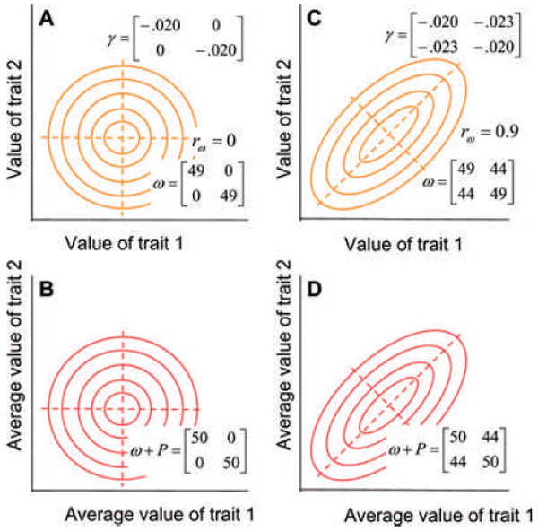
Individual selection surfaces and adaptive landscapes for two phenotypic traits can be represented by matrices or contour plots. The plots illustrate two kinds of bivariate stabilizing selection. Eigenvectors (principal components) are shown with dashed lines. The bivariate phenotypic mean is situated at the adaptive peak (intersection of the dashed lines) and consequently there is no directional selection. (A) An individual selection surface with weak stabilizing selection on each trait (γ11 = γ22 = −0.20) but no correlational selection (γ12 = 0). In this plot, expected individual fitness (contours) is a function of trait values. Because the curvature of this surface is weak, it can be approximated by a bivariate Gaussian surface described by the ω-matrix. (B) The adaptive landscape corresponding to the individual selection surface described in (A). In this plot, average population fitness (contours) is a function of average trait values. P is the within-population variance–covariance matrix before selection. The elements in the illustrated case are P11 = P22 = 1, P12 = P21 = 0. (C) An individual selection surface with weak stabilizing selection on each trait and positive correlational selection (ω12 = 44, _r_ω = 0.9). (D) The adaptive landscape corresponding to (C). The P-matrix is the same as in (B). Note that in these examples, the AL and the ISS have similar curvature and orientation because selection is weak (i.e., ω-matrix is large) relative to the P-matrix.
The AL for phenotypic traits can be used to represent many important features of evolution (Simpson 1944; Lande 1979, 2007; Arnold et al. 2001). The strength of stabilizing selection acting on the characters can be represented by the curvature of the landscape (Lande and Arnold 1983). Strong stabilizing selection is represented by a peak with steep slopes, whereas weak stabilizing selection is represented by a hilltop surrounded by gradual slopes. Correlational selection can be represented by ridges, corridors, or tubes in a multivariate landscape (Lande and Arnold 1983; Wagner 1984, 1988; Bürger 1986a,b; Phillips and Arnold 1989; Blows et al. 2004; Blows 2007). An important general property of the AL is that the population mean tends to evolve upwards on this surface, toward an adaptive peak (Lande 1979, 1980a). The departure of the phenotypic mean from an adaptive peak (e.g., because the mean drifts or the peak moves) induces directional selection, which causes the mean to evolve back toward the peak. The tempo of evolution can be captured by models of peak movement (Lande 1976a; Slatkin and Lande 1976; Bull 1987; Felsenstein 1988; Charlesworth 1993a,b; Lynch and Lande 1993; Bürger and Lynch 1995; Hansen and Martins 1996; Lande and Shannon 1996; Arnold et al. 2001). Long-term stability of peak position results in evolutionary stasis; the phenotypic mean evolves toward the stationary peak and remains in its vicinity. The mean evolves in a stochastic pattern about such a stationary peak if the population is of finite size, or if the peak itself moves stochastically about a particular point. Sustained movement of the peak in a particular direction results in phenotypic gradualism, as the mean tracks the trend in peak movement. Landscape dynamics can also be used to represent the ecological evens that underlie adaptive radiations, for example, invasions of predators or competitors or other kinds of environmental change that induce selection (Simpson 1944; Schluter 2000). Before leaving this survey we should mention that we have assumed that selection is frequency independent. When selection is frequency dependent, the tendency to maximize fitness and some other properties of the AL become problematic (Lande 2007).
It is useful to visualize both the AL and the ISS as surfaces with fitness contours and characteristic axes (Fig. 1). For the remainder of our review we will be concerned with a special case in which multivariate stabilizing selection is relatively weak, so that a single adaptive peak governs the deterministic behavior of the multivariate trait mean (In contrast, effective population size governs the stochastic behavior of the mean, in other words, its drift). Despite the simplicity of this vision, we will depart from the view of selection, introduced by Schmalhausen (1949) and Fisher (1958), in which the surface is portrayed as a circular, hill-shaped surface (Fig. 1A and 1B). In particular, we will allow for the possibility of correlational selection (selection that directly affects trait correlations within a generation), so that the surface is a ridge, tilted in trait space (Fig. 1C and 1D). Correlational selection is important because of the dominant role it plays in the evolution of phenotypic integration by shaping trait correlations (Lande 1980b). Finally, in a convention that will be important for the rest of our article, we will capture the essential features of the ridge and its orientation by drawing the principal components or eigenvectors of our bivariate surfaces (Fig. 1). The principal component (leading eigenvector) is oriented along the main axis of the ridge. (Associated with each eigenvector is an eigenvalue that measures the amount of curvature in that direction.) This leading axis (with the largest eigenvalue) defines a dimension in which fitness changes the least per unit change in the traits. In the case of a bivariate normal (Gaussian) ISS (Fig. 1), the largest eigenvalue is analogous to a variance; the larger the variance, the less fitness changes per unit change in the traits. We will refer to this dimension as the selective line of least resistance. An important significance of this dimension is that for many kinds of traits one can argue that peak movement is especially likely along this selective line (Arnold et al. 2001). We now turn to two entities that determine how the trait mean responds to the AL, the G- and M-matrices.
G- and M-matrices in Dynamic Equilibrium
The G-matrix is the central concept in understanding the inheritance of multiple traits, each of which is affected by many genes (Lande 1979; Arnold 1992; Lynch and Walsh 1998). Each individual in a population possesses a genetic value for each phenotypic trait that it transmits to its offspring (Fisher 1918). We can think of those genetic values as forming a statistical cloud that might be shaped like a soccer ball or a cigar (Fig. 2). We can represent the cloud with a G-matrix that consists of additive genetic variances for the traits on its main diagonal and set of additive genetic covariances between traits (arising from pleiotropy and linkage disequilibrium) as its off-diagonal elements (Fig. 2). Alternatively, assuming a normal (Gaussian) bivariate distribution of values, we can represent the cloud with a 95% confidence ellipse whose axes represent the principal components or eigenvectors of the G-matrix (Fig. 2). The length of each axis is determined by the corresponding eigenvalues of the G-matrix. (More exactly, the distance along each axis, from the center of the ellipse to its edge, is 1.96 times the square root of the corresponding eigenvalue). The longest axis of the ellipse (the leading eigenvector) is of particular interest because it represents the dimension in trait space for which there is the maximum amount of genetic variance. This dimension is sometimes called the genetic line of least resistance (Schluter 1996).
Figure 2.
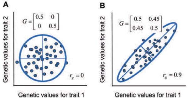
The distribution of additive genetic values for two traits can be represented as a cloud of values or a matrix, G. Same conventions as in Figure 2. (A) A data cloud with no genetic correlation (rg = 0). (B) A data cloud with a strong positive genetic correlation (rg = 0.9).
Thinking of the G-matrix as an ellipse, we can imagine the impact of opposing forces that buffet the G-ellipse each generation. For the moment our aim is to formulate an intuitive picture of this buffetting; we will treat the effects more formally later on. Selection, especially stabilizing selection, will nibble away at the cloud each generation. The immediate effects of such selection act within a generation and should tend to make the ellipse smaller, while possibly altering its shape and orientation. The biggest effects of selection should occur in those dimensions of the AL with the greatest curvature, for in those dimensions nibbling is the strongest. In contrast, finite sampling of parents each generation should on the average reduce the size of the ellipse without changing its shape or orientation. Mutation is the opposing process that counteracts the reducing/torquing effects of selection and drift. We can visualize the mutations that enter the population each generation at a particular locus as a sample from a cloud of pleiotropic values that can be represented either as a matrix (the M-matrix) or a 95% confidence ellipse (Fig. 3). The leading eigenvector of the M-matrix might be out of alignment with the main axis of the AL. In such a case at equilibrium, the AL torques the G-matrix in one direction each generation, while the input from mutation (and recombination) torques G in the opposite direction. We can imagine the G-ellipse at equilibrium stochastically rocking to and fro, while pulsating in size and shape under the opposing forces of selection, drift, and mutation. At another extreme, this wobbling and pulsating of the G-ellipse might be quite small should the main axes of the AL and M-matrix happen to be aligned.
Figure 3.
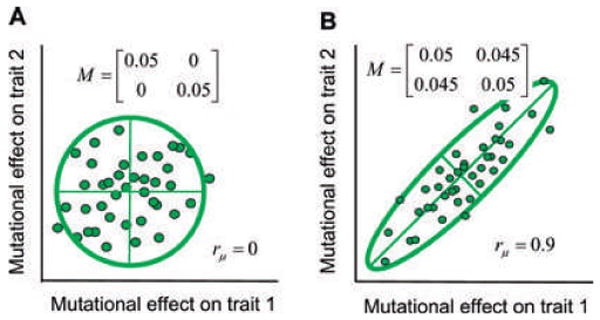
The distribution of new mutational effects on two traits from a particular locus can be represented as a cloud of values or a matrix, M. The 95% confidence ellipses for each data cloud are shown. The axes inside each ellipse are eigenvectors (principal components). (A) A cloud of mutations with no correlation (_r_μ = 0). (B) A cloud of mutations with a strong positive correlation in mutational effects (_r_μ = 0.9).
It is important to realize that G might change on three timescales. In the preceding discussion we focused on a short, within-generation timescale. Within generations, G pulsates and wobbles in response to opposing forces, even after it has equlibrated to those forces. On a longer timescale, G might evolve in response to a change in selection regime (e.g., a new AL) and attain a new equilibrium state. If we think of the M-matrix as a constant, for the moment, then we might imagine the newly equilibrated G-ellipse to represent a compromise between the AL and the M-ellipse. In particular, the leading eigenvector of G should be intermediate between the leading eigenvectors of the AL and M. On the other hand, the shape of G might be fatter or narrower than M depending on the multivariate curvature of the AL. Finally, let us relax our assumption that the M-matrix is constant. Just as G might evolve in response to the AL, so might M. Although we might expect M to evolve toward alignment (shared eigenvectors) with the AL, we should also expect that evolution to be slower than the evolution of G for a simple reason. The genetic values summarized by G make a direct contribution to the phenotypic values of an individual. In contrast, the mutational tendencies summarized by M contribute to phenotypic values more rarely (by 2–4 orders of magnitude!) and even when they do contribute, their average effect is small. In summary G fluctuates on a very short timescale and evolves on both an intermediate timescale (on which M is effectively constant) and a long timescale (during which M itself might evolve). When we turn to the results of simulation studies, in a later section, we will explore the stability and evolution of G on all three of these timescales.
Importance of the G-matrix and Its Stability
The G-matrix plays a crucial role in formal theory for the evolution of polygenic traits, including the population's evolutionary response to the AL. The G-matrix profoundly affects response of the phenotypic mean to selection (Lande 1979). G can also be used to reconstruct historical patterns of selection and to test genetic drift as a null model for differentiation (Lande 1979; Jones et al. 2004; Hohenlohe and Arnold 2008). In all three contexts, stability of the G-matrix is an important but unresolved problem. Because the G-matrix is bound to fluctuate in a population of finite size (Lande 1979), the question of stability does not have a simple yes or no answer. Instead we must consider a set of more subtle issues. What types of quantitative characters have relatively stable G-matrices and over what timescale? Are some aspects of G-matrix structure more stable than others? How much are evolutionary inferences affected by systematic and random changes in the G-matrix? Although the importance of these issues is both apparent and widely acknowledged, we have so far been unable to settle them with the analytical machinery of algebra and calculus.
Analytical Studies of G-matrix Evolution and Stability
The theoretical characterization of the G-matrix after it has equilibrated under a static regime of selection, mutation, and recombination has only been achieved under various sets of simplifying assumptions. These assumptions include additivity of genetic effects, linkage equilibrium, and infinite population size. Analytical approximations for the magnitude of the constituent variances and covariances at mutation–selection balance have been obtained for only a narrow range of conditions denned by simplifying assumptions such as a multivariate Gaussian distribution of allelic effects (Lande 1976b, 1980b; Turelli and Barton 1990), mutational effects that are much larger than the standing genetic variation (Turelli 1985), and a certain model of constrained pleiotropic effects (Wagner 1989). For finite populations, no theoretical predictions for the multivariate case have yet been derived. In addition, we do not have equations for the generation-by-generation dynamics of the evolving G-matrix, except under very special assumptions (Turelli 1985). Even in the case of a single character, these issues are fairly complex, and it has been shown that the dynamics of the genetic variance depends upon the higher moments of the distribution of allelic effects as well as on other genetic details (Barton and Turelli 1989; Bürger 2000). Consequently, we cannot predict how much the G-matrix will wobble and pulsate due to the interaction of genetic drift with selection, mutation, and recombination, even if the AL remains constant. For all these reasons, the evolution and stability of the G-matrix have been viewed as empirical issues (Turelli 1988) and pursued as such over the last 25 years (Steppan et al. 2002).
Empirical Studies of G-matrix Evolution and Stability
Various techniques for comparing G-matrices have been proposed and each has strengths and weaknesses (Steppan et al. 2002). We will summarize the empirical work using just one of these techniques, the Flury hierarchy, because the format for comparisons can be easily related to the analytical and simulation work on the G-matrix (see Houle et al. 2002 for a discussion of limitations). The Flury hierarchy is based on comparisons of eigenvectors and eigenvalues (Flury 1988; Phillips and Arnold 1999; Arnold and Phillips 1999). A useful feature of this approach is that these comparisons can be arranged in a hierarchy of tests (Fig. 4) that range from a test for equal matrices (identical eigenvectors and eigenvalues) to a test for unrelated matrices (dissimilar eigenvectors and eigenvalues). As we will see, G-matrix comparisons often fall in the intermediate territory in which some or all eigenvectors are equal but eigenvalues are dissimilar.
Figure 4.
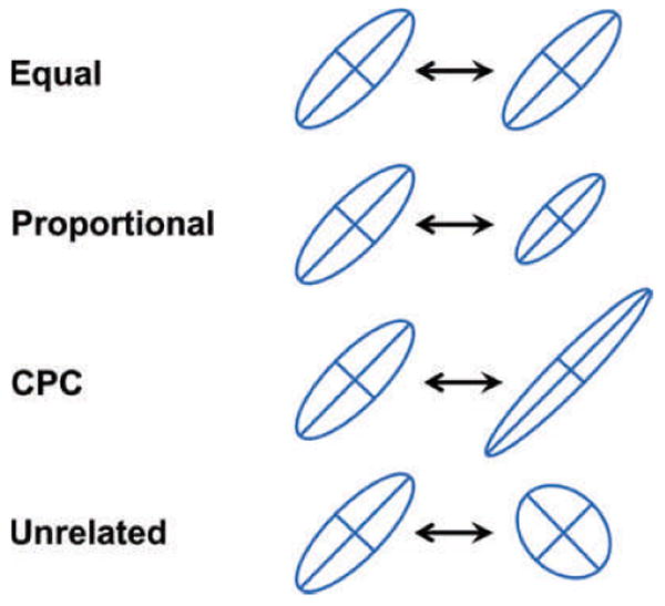
The Flury hierarchy for comparing G-matrices is a nested series of hypotheses that are tested by comparing eigenvectors and eigenvalues. The hypotheses are listed on the left and depicted on the right with 95% confidence ellipses. From top to bottom, the hypotheses are: (A) equal matrices (eigenvectors equal, eigenvalues equal), (B) proportional matrices (eigenvectors equal; eigenvalues proportional), (C) matrices with common principal components, CPC (eigenvectors equal, eigenvalues not equal), and (D) unrelated matrices (eigenvectors and eigenvalues not equal). For more than n = 2 traits, an additional possible hypothesis is partial CPC, in which up to n − 2 eigenvectors are shared among matrices, but the remaining eigenvectors differ.
The predominant empirical approach has been to compare matrices sampled from nature or from experimental treatments, each of which has strengths and weaknesses (Phillips and McGuigan 2006). A strength of comparing matrices from natural populations is that the results are likely to reflect configurations under natural conditions. The histories of selection and population size may be unknown, but at least they are representative of the real world. A limitation in nonexperimental work is that usually only two or three matrices are available for comparison, because of the difficulty of assembling the large samples of families needed to estimate G. On the experimental side, G-matrices have been compared after separate subpopulations have been exposed to different mutagens, allowed to drift, or grown under different rearing conditions. A strength of the approach is that the nature of the treatments is known. A limitation is that some natural forces that normally promote eigenvector stability may be missing. Nevertheless, comparative work of this kind has revealed some intriguing results.
G-matrices sampled from experimental and natural populations often show conserved aspects of structure. In particular, the eigenvectors (principal components) of the matrix often are conserved (Fig. 5). A large proportion of the comparisons that have been made show similarity in eigenvectors (equal, proportional, partial CPC, or full CPC). In comparisons of experimental treatments, sexes, conspecific populations, and different species the proportion of comparisons with similar eigenvectors is 78%, 75%, 74%, and 78%, respectively (see http;//oregonstate.edu/∼arnoldst/Gcomparisons/index.htm for more details and a list of references). A survey of 35 additional studies that compared G-matrices of different conspecific populations and species using other methods yielded similar results. Evidence of matrix similarity was found in 74% of those studies. Despite this strong signal of stability across diverse comparisons, a variety of studies have also shown that selection, such as that associated with character displacement and adaptive radiations, can lead to differences in G, even over short timescales (Fong 1989; Jernigan et al. 1994; Van 'T Land et al. 1999; Roff 2002; Roff et al. 2004; Cano et al. 2004; McGuigan et al. 2005; Doroszuk et al. 2008). Experiments have also established that the G-matrix can wobble, inflate, and contract in the absence of selection, especially in small populations (Phillips et al. 2001).
Figure 5.
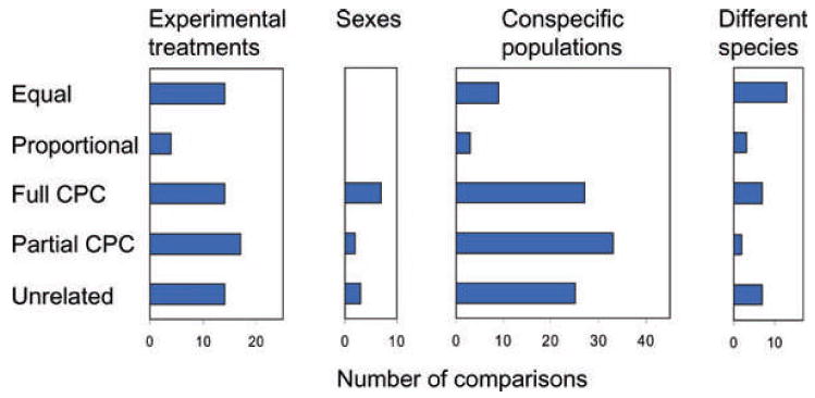
Graphical summary of the results of empirical comparisons of G-matrices. Only 31 studies that made comparisons with the Flury hierarchy are included here. From left to right, the four panels refer to studies that compared experimental populations of the same species that have been exposed to different environmental treatments (n = 63 pairwise comparisons), males and females from the same population (n = 12), conspecific populations sampled from nature (n = 97), or different species sampled from nature (p = 32). The outcomes of statistical tests are classified into categories described in Figure 4. Full CPC means that matrices had all principal components (eigenvectors) in common) partial CPC means at least one but not all principal components are in common. Some studies compared multiple pairs of matrices. In such cases, all of the outcomes are tabulated.
Although computer simulations of evolving G-matrices do not solve all of the problems that plague empirical comparisons and their interpretation, they do offer a complementary approach to the problems of G-matrix evolution and stability. In particular, simulation studies can help us understand the forces responsible for eigenvector stability in comparative studies, as well as the erratic wobbling of the matrix that can occur when selection is experimentally removed.
Simulation Studies of G-matrix Evolution and Stability
Several studies have used a simulation-based approach to study various aspects of quantitative trait evolution (Bürger et al. 1989; Wagner 1989; Bürger and Lande 1994; Baatz and Wagner 1997; Wagner et al. 1997; Reeve 2000), but only recently has this approach focused specifically on G-matrix evolution and stability (Jones et al. 2003, 2004; Guillaume and Whitlock 2007; Jones 2007; Revell 2007). To make this approach practical, usually one studies only two traits, each affected by 10–100 pleiotropic loci. Despite these limitations, the programs simulate processes of mutation, selection, population regulation, and inheritance in populations of hundreds to thousands of individuals over thousands of generations. An important feature of these simulation programs is that–so far as is possible–their parameter values are anchored in actual data. The programs are designed so that their parameters mesh with available analytical theory, enabling both cross-checking of results and realistic choices of values for descriptors of mutation, selection, inheritance, population size, and peak movement by reference to empirical surveys (Endler 1986; Mousseau and Roff 1987; Kingsolver et al. 2001–see Jones et al. 2003; Estes and Arnold 2007). A consistent result with these simulation programs is that they confirm theoretical predictions about the evolution of the phenotypic mean. For example, the trait mean does evolve toward an optimum, and it tracks a moving optimum with the theoretically predicted degree of lag. The main goal in the new genre of simulation studies is to answer questions about G and M that cannot be answered with available theory.
In the first study in this new simulation genre, Jones et al. (2003) examined the evolution and stability of the G-matrix in response to a stabilizing AL that is constant both in configuration and position. Focusing first on the shortest time scale, within generations, one of the main findings was that different aspects of stability react differently to selection, mutation, and drift. In particular, small population size is a key factor causing fluctuations in eigenvalues and their proportionality. In contrast, correlational selection (large _r_ω) and pleiotropic mutation (large _r_μ), as well as large population size promote stability of the eigenvectors of the G-matrix (Fig. 6). Eigenvector stability is especially enhanced if correlational selection and pleiotropic mutation are not only strong but have the same sign (i.e., aligned eigenvectors) (Jones et al. 2003). Under these conditions, stability is retained even if the position of the optimum fluctuates randomly from generation to generation (Revell 2007).
Figure 6.
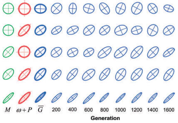
Evolution and stability of the G-matrix in response to different patterns of mutation and selection (stationary optimum). Each row shows the results (snapshots) from a single simulation run lasting 2000 generations. The first three ellipses in each row are the 95% confidence ellipses (or equivalent) for the M-matrix, the adaptive landscape (ω + P matrix), and the resulting average G-matrix (n = 2000 generations). These three ellipses are shown on different scales. The average G-matrix is the reference size, but the M-matrix is magnified by a factor of 3, and the ω + P matrix is reduced by a factor of 10. The average P-matrix (n = 2000 generations) was added to the ω-matrix to compute the ω + P matrix. The last eight ellipses in each row show snapshots of the G-matrix (95% confidence ellipses) every 200 generations, shown at the same scale as the average G-matrix. From top to bottom, the values of mutation and selection and the resulting average genetic correlation are: (A) _r_μ = _r_ω = 0, _r_g = −0.09. (B) _r_μ = 0, _r_ω = 0.75, _r_g = 0.29. (C) _r_μ = 0.50, _r_ω = 0, _r_g = 0.48. (D) _r_μ = 0.50, _r_ω = 0.75, _r_g = 0.64. (E) _r_μ = 0.90, _r_ω = 0.90, _r_g = 0.93. The following parameters are the same for all rows: _N_e = 342, ω11 = ω22 = 49, and the mutational variances for each character are 0.05 (as in Fig. 3).
Focusing on a longer time scale, we find that the G-matrix evolves in expected ways to the AL and the pattern of mutation. In the absence of correlational selection (_r_ω = 0) and mutational correlation (rμ = 0), the average G-ellipse is nearly circular, although the ellipse fluctuates wildly about this average (first row in Fig. 6). At the opposite extreme, when the leading eigenvectors of the AL and the M- matrix are both inclined at an angel of 45°, the leading eigenvector of G is pitched at the same angle (last row in Fig. 6). Between these two extremes, G tends to evolve to a shape and orientation that represents an intermediate compromise between the AL and M. In other words, the simulation results confirm our intuition and theoretical expectations (Lande 1980b) that G should evolve toward alignment with the AL and M.
These results allow us to interpret the features of conservation observed in comparative studies of actual G-matrices. In small simulated populations, and in the absence of restraining factors, the G-matrix fluctuates wildly in size and orientation. Both the eigenvalues and the eigenvectors of the matrix are unstable. Thus, the stability of the G-matrix that has commonly been observed in comparative studies should not be taken for granted. It must arise from a factor or set of factors that confer stability. The Jones et al. (2003) simulation study suggests that this set of factors includes large population size, as well as strong, persistent, and coordinated patterns of correlational selection and pleiotropic mutation. The fact that eigenvector stability of G-matrices is so frequently observed suggests that this set of circumstances is common in nature. We will return to the issue of coordinated patterns of mutation and selection later in this article.
In another study, Jones et al. (2004) allowed the adaptive peak to move while the landscape itself maintained a constant configuration (Fig. 7). This model of selection corresponds to temporal change in the environment or the invasion of a new adaptive zone (Simpson 1944). The addition of a moving optimum yielded several important new insights. First, evolution along a selective line of least resistance (i.e., along the eigenvector corresponding to the leading eigenvalue of the AL) increased stability of the orientation of the G-matix relative to stabilizing selection alone (Fig. 7B). Evolution perpendicular to genetic lines of least resistance decreased G-matrix stability. Second, evolution in response to a continuously changing optimum can produce persistent mal-adaptation for correlated traits, because the evolving mean never catches up with the moving optimum. Furthermore, when the optimum for one trait moves, but the optimum for the other trait does not, the mean of that second trait can be permanently displaced from its optimum as a consequence of correlated responses to selection. Overall, these results show that directional selection actually can increase stability of the G-matrix.
Figure 7.
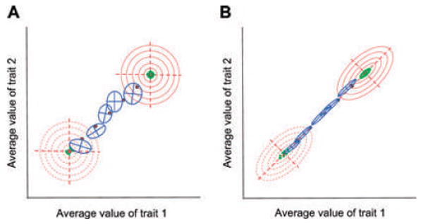
Contrasting conditions can promote instability or stability of the G-matrix on an adaptive landscape with a moving optimum. Results from simulations using the Jones et al. (2004) program are shown in this figure. In both cases the peak of the adaptive landscape (solid red dot) has moved from the bottom left to the upper right at the same rate. Peak position is shown every 300 generations. The bivariate phenotypic mean (intersection of the axes of the G-matrix, shown as a blue ellipse) tracks the moving peak and is also shown every 300 generations. Effective population size is relatively small (_N_e = 342). (A) No correlated pleiotropic mutational effects (shown as a circular green ellipse, _r_μ = 0) and no correlational selection (shown as a circular adaptive landscape, red contours, _r_ω = 0) promote instability of the G-matrix. Notice that G (blue ellipses) changes in size, shape, and especially in orientation from snapshot to snapshot. (B) Strong mutational correlation (_r_μ = 0.9) and strong correlational selection (_r_ω = 0.9), combined with peak movement along the selective line of least resistance, promote stability in the size, shape, and orientation of the G-matrix. Notice that the cigar-shaped G-matrices hardly vary from snapshot to snapshot. Although the three stability-promoting conditions are combined here, other simulations show that they make individual contributions to the stability and evolution of the G-matrix.
Guillaume and Whitlock (2007) have shown that strong migration can also affect G-matrix evolution and stability. Consider the case of an island population that receives migrants from a larger mainland population with a different adaptive peak. The effects of migration depend on its strength and the direction of peak movement. Strong migration can stabilize the G-matrix if peak movement during island–mainland differentiation is along a selective line of least resistance. In this case, migration can exaggerate the cigar shape of the G-matrix. Destabilization by migration is also possible if peak movement is perpendicular to the selective line of least resistance. In this case, a cigar-shaped G-matrix can be fattened and rotated by migration.
Stability and Evolution of the G-matrix When Mutational Effects Evolve
In the simulation studies discussed so far, the evolution of G was constrained because the process of mutation was not allowed to evolve. If we allow M to evolve, we might expect it to evolve toward alignment with the AL (Lande 1980b; Jones et al. 2007). In a simplified approach with two characters, Jones et al. (2007) found that even though the M-matrix experiences extremely weak selection, it does indeed evolve in response to the AL in predictable ways. In particular, the M-matrix tends to evolve toward alignment with the AL (Fig. 8). This result is important because it indicates that the M-matrix, like the G-matrix, can be shaped by the AL. Furthermore, an evolving M-matrix confers greater stability on G than does a static mutational process. Thus, this recent study increases optimism that G-matrix stability may be a firmly rooted empirical reality.
Figure 8.
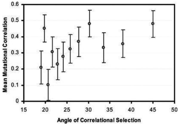
The M-matrix tends to evolve toward alignment with the adaptive landscape. This figure summarizes the results of simulations in which one feature of the M-matrix, the mutational correlation (_r_μ), was allowed to evolve as the orientation of the adaptive landscape was varied. In different runs the selectional correlation (_r_ω) was held constant at 0.90 by systematically varying the elements of the ω-matrix, so that the orientation of the leading eigenvector of the adaptive landscape (angle of correlational selection) varied from about 19–45 degrees (replotting of data shown in Fig. 5 of Jones et al. 2007). Each point represents the mean of 50 replicate runs (± SE).
At the same time, additional simulation studies are needed that will move past the simplifying assumptions used in the first round. The approach of Jones et al. (2007) was simplified by assuming that gene effects were purely additive and variation in the mutation process was contrived in the sense that it did not arise naturally from genetic architecture. In real genetic systems, variation in pleiotropic mutation arises from nonadditive interactions between genes (epistasis) (Cheverud 1996; Hermisson et al. 2003; Carter et al. 2005). Thus, a current challenge is to understand how the G- and M-matrices evolve in more realistic systems of genetic architecture that include dominance and epistasis.
Conclusions
Our review of theoretical and empirical work on G-matrix stability and evolution reveals several results that could shape new methodologies for analyzing adaptive radiations. One important result is supported by empirical, analytical, and simulation studies. The G-matrices of characters under multivariate stabilizing selection in large populations may be relatively stable in size and shape and show a stable orientation that is aligned with the AL. Theoretical work, for instance, indicates that alignment between G and the AL is produced directly by stabilizing and correlational selection and indirectly as the M-matrix evolves toward alignment with the landscape. Furthermore, the simulation studies indicate that movement of the adaptive peak can confer additional stability on the orientation (eigenvectors) of the G-matrix, especially when that movement is aligned with the leading eigenvector of the landscape. These results are important because they identify a class of phenotypic characters whose adaptive radiations can be analyzed by assuming relative constancy of the G-matrix.
Our review also reveals three important, unresolved issues in phenotypic evolution that may hold the key to understanding the five emerging generalizations listed at the start of this article. First, long-term persistence in the configuration of the AL seems likely on several grounds (Estes and Arnold 2007) and could produce persistent, coordinated patterns of both pleiotropic mutation and inheritance (Arnold et al. 2001; Jones et al. 2007). Although landscape persistence seems plausible, the jury is still out on this important empirical issue. Comparative studies of the AL are still so rare that we may have to settle for indirect evidence for persistence. Thus, the patterns of stasis and constrained trait divergence that have been regularly observed in the fossil record are telling because they suggest persistent stabilizing selection (Estes and Arnold 2007). Second, the simulation work indicates that the structural stability of the G-matrix that has regularly been observed in comparative studies could arise from alignment of G with persistent ALs. Here again is an unresolved empirical question, one that will require comparing G with ALs. Third, the simulation studies have also shown that the evolution and stability of G is affected by the direction of movement of the adaptive peak. On first principles one can argue that peak movement is likely to occur along selective lines of least resistance (Arnold et al. 2001). Once again, the jury is out. We urgently need more case studies in which the co-evolutionary pattern of means of multiple populations or species can be compared with the pattern of selection within populations (Hohenlohe and Arnold 2008).
Supplementary Material
Figure 5 references
G-matrix comparisons
Acknowledgments
We thank S. Estes, J. Hermisson, P. C. Phillips, L. Revell, and two anonymous reviews for discussion and comments on an earlier version of this article. The preparation of this manuscript was supported by the U.S. National Science Foundation (grant DEB-0047554 to SJA and RB and grant DEB-0044268 to AGJ), a U.S. National Institutes of Health Ruth L. Kirschstein National Research Service Award Fellowship to PAH, and an AGEP Fellowship to BCA.
Literature Cited
- Arnold SJ. Constraints on phenotypic evolution. Am Nat. 1992;140:S85–S107. doi: 10.1086/285398. [DOI] [PubMed] [Google Scholar]
- Arnold SJ, Phillips PC. Hierarchical comparison of genetic variance covariance matrices. II. Coastal-inland divergence in the garter snake, Thamnophis elegans. J Evol Biol. 1999;53:1516–1527. doi: 10.1111/j.1558-5646.1999.tb05415.x. [DOI] [PubMed] [Google Scholar]
- Arnold SJ, Pfrender ME, Jones AG. Tire adaptive landscape as a conceptual bridge between micro- and macroevolution. Genetica. 2001:112–113. 9–32. [PubMed] [Google Scholar]
- Baatz M, Wagner GP. Adaptive inertia caused by hidden pleiotropic effects. Theor Pop Biol. 1997;5:49–66. [Google Scholar]
- Barton N, Keightley PD. Understanding quantitative genetic variation. Nat Rev Genet. 2002;3:11–20. doi: 10.1038/nrg700. [DOI] [PubMed] [Google Scholar]
- Barton NH, Turelli M. Evolutionary quantitative genetics-how little do we know? Annu Rev Genet. 1989;23:337–370. doi: 10.1146/annurev.ge.23.120189.002005. [DOI] [PubMed] [Google Scholar]
- Blows MW. A tale of two matrices: multivariate approaches in evolutionary biology. J Evol Biol. 2007;20:1–8. doi: 10.1111/j.1420-9101.2006.01164.x. [DOI] [PubMed] [Google Scholar]
- Blows M, Hoffman A. A reassessment of genetic limits to evolutionary change. Ecology. 2005;86:1371–1384. [Google Scholar]
- Blows M, Chenoweth SF, Hine EJ. Orientation of the genetic variance-covariance matrix and the fitness surface for multiple male sexually selected traits. Am Nat. 2004;163:329–340. doi: 10.1086/381941. [DOI] [PubMed] [Google Scholar]
- Brodie ED, III, Moore DJ, Janzen FJ. Visualizing and quantitfying natural selection. Trends Ecol Evol. 1995;10:313–318. doi: 10.1016/s0169-5347(00)89117-x. [DOI] [PubMed] [Google Scholar]
- Bull JJ. Evolution of phenotypic variance. Evolution. 1987;41:303–315. doi: 10.1111/j.1558-5646.1987.tb05799.x. [DOI] [PubMed] [Google Scholar]
- Bürger R. Constraints for the evolution of functionally coupled characters: a nonlinear analysis of a phenotypic model. Evolution. 1986a;40:182–193. doi: 10.1111/j.1558-5646.1986.tb05729.x. [DOI] [PubMed] [Google Scholar]
- Bürger R. Evolutionary dynamics of functionally constrained phenotypic characters. IMA J Math Appl Med Biol. 1986b;3:265–287. [PubMed] [Google Scholar]
- Bürger R. The mathematical theory of selection, recombination, and mutation. Wiley; New York, NY: 2000. [Google Scholar]
- Bürger R, Lande R. On the distribution of the mean and variance of a quantitative trait under mutation-selection-drift balance. Genetics. 1994;138:901–912. doi: 10.1093/genetics/138.3.901. [DOI] [PMC free article] [PubMed] [Google Scholar]
- Bürger R, Lynch M. Evolution and extinction in a changing environment: a quantitative genetic analysis. Evolution. 1995;49:151–163. doi: 10.1111/j.1558-5646.1995.tb05967.x. [DOI] [PubMed] [Google Scholar]
- Bürger R, Wagner GP, Stettinger J. How much heritable variation can be maintained in finite populations by mutation-selection balance. Evolution. 1989;43:1748–1766. doi: 10.1111/j.1558-5646.1989.tb02624.x. [DOI] [PubMed] [Google Scholar]
- Cano JM, Laurila A, Palo J, Media J. Population differentiation in G matrix structure due to natural selection in Rana temporaria. Evolution. 2004;58:2013–2020. doi: 10.1111/j.0014-3820.2004.tb00486.x. [DOI] [PubMed] [Google Scholar]
- Carter AJR, Hemrisson J, Hansen TF. The role of epistatic gene interactions in the response to selection and the evolution of evolvability. Theor Pop Biol. 2005;68:179–196. doi: 10.1016/j.tpb.2005.05.002. [DOI] [PubMed] [Google Scholar]
- Charlesworth B. Directional selection and the evolution of sex and recombination. Genet Res. 1993a;61:205–224. doi: 10.1017/s0016672300031372. [DOI] [PubMed] [Google Scholar]
- Charlesworth B. The evolution of sex and recombination in a varying environment. J Heredity. 1993b;84:345–350. doi: 10.1093/oxfordjournals.jhered.a111355. [DOI] [PubMed] [Google Scholar]
- Charlesworth B, Lande R, Slatkin M. A neo-Darwinian commentary on macroevolution. Evolution. 1982;36:474–98. doi: 10.1111/j.1558-5646.1982.tb05068.x. [DOI] [PubMed] [Google Scholar]
- Cheverud JM. Developmental integration and the evolution of pleiotropy. Am Zool. 1996;36:44–50. [Google Scholar]
- Doroszuk A, Wojewodzic MW, Gort G, Kammenga JE. Rapid divergence of genetic variance-covariance matrix within a natural population. Am Nat. 2008;171:291–304. doi: 10.1086/527478. [DOI] [PubMed] [Google Scholar]
- Endler JA. Natural selection in the wild. Princeton Univ Press; Princeton, NJ: 1986. [Google Scholar]
- Estes S, Arnold SJ. Resolving the paradox of stasis: models with stabilizing selection explain evolutionary divergence on all timescales. Am Nat. 2007;169:227–244. doi: 10.1086/510633. [DOI] [PubMed] [Google Scholar]
- Felsenstein J. Phylogenies and quantitative characters. Ann Rev Ecol Syst. 1988;19:445–471. [Google Scholar]
- Fisher RA. The correlation between relatives on the supposition of Mendelian inheritance. Trans R Soc Edinburgh. 1918;52:399–433. [Google Scholar]
- Fisher RA. The genetical theory of natural selection. Dover; New York, NY: 1958. [Google Scholar]
- Flury BD. Common principal components and related multivariate models. Wiley; New York, NY: 1988. [Google Scholar]
- Fong DW. Morphological evolution of the amphipod Gammarus minus in caves: quantitative genetic analysis. Am Midl Nat. 1989;121:361–378. [Google Scholar]
- Gould SJ. Allometry and size in ontogeny and phylogeny. Biol Rev Camb Phil Soc. 1966;41:587–640. doi: 10.1111/j.1469-185x.1966.tb01624.x. [DOI] [PubMed] [Google Scholar]
- Gould SJ. The structure of evolutionary theory. Harvard Univ Press, Boston, MA 2002 [Google Scholar]
- Guillaume F, Whitlock MC. Effects of migration on the genetic covariance matrix. J Evol Biol. 2007;61:2398–2409. doi: 10.1111/j.1558-5646.2007.00193.x. [DOI] [PubMed] [Google Scholar]
- Hairston NG, Jr, Ellner SP, Geber MA, Yoshida T, Fox JA. Rapid evolution and the convergence of ecological and evolutionary time. Ecol Lett. 2005;8:1114–1127. [Google Scholar]
- Hansen TF, Martins EP. Translating between microevolutionary process and macroevolutionary patterns: the correlation structure of interspecific data. Evolution. 1996;50:1404–1417. doi: 10.1111/j.1558-5646.1996.tb03914.x. [DOI] [PubMed] [Google Scholar]
- Harvey PH, Pagel MD. The comparative method in evolutionary biology. Oxford Univ Press; Oxford, UK: 1991. [Google Scholar]
- Hermisson J, Hansen TF, Wagner GP. Epistasis in polygenic traits and the evolution of genetic architecture. Am Nat. 2003;161:708–734. doi: 10.1086/374204. [DOI] [PubMed] [Google Scholar]
- Hohenlohe PA, Arnold SJ. MIPod: a hypothesis testing framework for microevolutionary inference from patterns of divergence. Am Nat. 2008;171:366–385. doi: 10.1086/527498. [DOI] [PMC free article] [PubMed] [Google Scholar]
- Houle D. Comparing evolvability and variability of quantitative traits. Genetics. 1992;130:195–204. doi: 10.1093/genetics/130.1.195. [DOI] [PMC free article] [PubMed] [Google Scholar]
- Houle D, Mezey J, Galpern P. Interpretation of the results of partial principal components analysis. Evolution. 2002;56:433–440. doi: 10.1111/j.0014-3820.2002.tb01356.x. [DOI] [PubMed] [Google Scholar]
- Jernigan RW, Culver DC, Fong DW. The dual role of selection and evolutionary history as reflected in genetic correlations. J Evol Biol. 1994;48:587–596. doi: 10.1111/j.1558-5646.1994.tb01346.x. [DOI] [PubMed] [Google Scholar]
- Jones AG, Arnold SJ, Burger R. Stability of the G-matrix in a population experiencing stabilizing selection, pleiotropic mutation, and genetic drift. Evolution. 2003;57:1747–1760. doi: 10.1111/j.0014-3820.2003.tb00583.x. [DOI] [PubMed] [Google Scholar]
- Jones AG, Arnold SJ, Burger R. Evolution and stability of the G-matrix on a landscape with a moving optimum. Evolution. 2004;58:1639–1654. doi: 10.1111/j.0014-3820.2004.tb00450.x. [DOI] [PubMed] [Google Scholar]
- Jones AG, Arnold SJ, Burger R. The mutation matrix and the evolution of evolvability. Evolution. 2007;61:727–745. doi: 10.1111/j.1558-5646.2007.00071.x. [DOI] [PubMed] [Google Scholar]
- Kingsolver JG, Hoekstra HE, Hoekstra JM, Berrigan D, Vignieri SN, Hill CE, Hoang A, Gilbert P, Beerlio P. The strength of phenotypic selection in natural populations. Am Nat. 2001;157:245–261. doi: 10.1086/319193. [DOI] [PubMed] [Google Scholar]
- Lande R. Natural selection and random genetic drift in phenotypic evolution. Evolution. 1976a;30:314–334. doi: 10.1111/j.1558-5646.1976.tb00911.x. [DOI] [PubMed] [Google Scholar]
- Lande R. The maintenance of genetic variability by mutation in a polygenic character with linked loci. Genet Res. 1976b;26:221–235. doi: 10.1017/s0016672300016037. [DOI] [PubMed] [Google Scholar]
- Lande R. Quantitative genetic analysis of multivariate evolution, applied to brain-body size allometry. Evolution. 1979;33:402–416. doi: 10.1111/j.1558-5646.1979.tb04694.x. [DOI] [PubMed] [Google Scholar]
- Lande R. Sexual dimorphism, sexual selection, and adaptation in polygenic characters. Evolution. 1980a;34:292–305. doi: 10.1111/j.1558-5646.1980.tb04817.x. [DOI] [PubMed] [Google Scholar]
- Lande R. The genetic covariance between characters maintained by pleiotropic mutation. Genetics. 1980b;94:203–215. doi: 10.1093/genetics/94.1.203. [DOI] [PMC free article] [PubMed] [Google Scholar]
- Lande R. Expected relative fitness and the adaptive topography of fluctuating selection. Evolution. 2007;61:1835–1846. doi: 10.1111/j.1558-5646.2007.00170.x. [DOI] [PubMed] [Google Scholar]
- Lande R, Arnold SJ. The measurement of selection on correlated characters. Evolution. 1983;37:10–1226. doi: 10.1111/j.1558-5646.1983.tb00236.x. [DOI] [PubMed] [Google Scholar]
- Lande R, Shannon S. The role of genetic variation in adaptation and population persistence in a changing environment. Evolution. 1996;50:434–437. doi: 10.1111/j.1558-5646.1996.tb04504.x. [DOI] [PubMed] [Google Scholar]
- Lynch M, Lande R. Evolution and extinction in response to environmental change. In: Kareiva P, Kingsolver JG, Huey RB, editors. Biotic Interactions and Global Change. Sinauer Associates; Sunderland, MA: 1993. pp. 234–250. [Google Scholar]
- Lynch M, Walsh B. Genetics and analysis of quantitative traits. Sinauer Associates; Sunderland, MA: 1998. [Google Scholar]
- Marroig G, Cheverud JM. Did natural selection or genetic drift produce cranial diversification of Neotropical monkeys? Am Nat. 2004;163:417–428. doi: 10.1086/381693. [DOI] [PubMed] [Google Scholar]
- McGuigan K, Chenoweth SF, Blows MW. Phenotypic divertgence along lines of genetic variance. Am Nat. 2005;165:32–43. doi: 10.1086/426600. [DOI] [PubMed] [Google Scholar]
- Mousseau TA, Roff DA. Natural selection and the heritability of fitness components. Heredity. 1987;59:181–197. doi: 10.1038/hdy.1987.113. [DOI] [PubMed] [Google Scholar]
- Phillips PC, Arnold SJ. Visualizing multivariate selection. Evolution. 1989;43:1209–1222. doi: 10.1111/j.1558-5646.1989.tb02569.x. [DOI] [PubMed] [Google Scholar]
- Phillips PC, Arnold SJ. Hierarchical comparison of genetic variance covariance matrices. I. Using the Flury hierarchy. Evolution. 1999;53:1506–1515. doi: 10.1111/j.1558-5646.1999.tb05414.x. [DOI] [PubMed] [Google Scholar]
- Phillips PC, McGuigan KL. Evolution of genetic variance-covariance structure. In: Fox CW, Wolf JB, editors. Evolutionary genetics: concepts and case studies. Oxford Univ Press; Oxford, England: 2006. pp. 310–325. [Google Scholar]
- Phillips PC, Whitlock MC, Fowler K. Inbreeding changes the shape of the genetic covariance matrix in Drosopilla melanogaster. Genetics. 2001;158:1137–1145. doi: 10.1093/genetics/158.3.1137. [DOI] [PMC free article] [PubMed] [Google Scholar]
- Reeve JP. Predicting long-term response to selection. Genet Res. 2000;75:83–94. doi: 10.1017/s0016672399004140. [DOI] [PubMed] [Google Scholar]
- Revell LJ. The G matrix under fluctuation correlational mutation and selection. Evolution. 2007;61:1857–1872. doi: 10.1111/j.1558-5646.2007.00161.x. [DOI] [PubMed] [Google Scholar]
- Roff DA. Comparing G matrices: a MANOVA approach. Evolution. 2002;56:1286–1291. [PubMed] [Google Scholar]
- Roff DA, Mousseau T, MØller AP, de Lope F, Saino N. Geographic variation in the G matrices of wild populations of the barn swallow. Heredity. 2004;93:8–14. doi: 10.1038/sj.hdy.6800404. [DOI] [PubMed] [Google Scholar]
- Schluter D. Adaptive radiation along genetic lines of least resistance. J Evol Biol. 1996;50:1766–1774. doi: 10.1111/j.1558-5646.1996.tb03563.x. [DOI] [PubMed] [Google Scholar]
- Schluter D. The ecology of adaptive radiation. Oxford Univ Press; Oxford, UK: 2000. [Google Scholar]
- Schmalhausen II. Factors of evolution, the theory of stabilizing selection. Univ of Chicago Press; Chicago, IL: 1949. [Google Scholar]
- Simpson GG. Tempo and mode in evolution. Columbia Univ Press; New York, NY: 1944. [Google Scholar]
- Slatkin M, Lande R. Niche width in a fluctuating environment–density independent model. Am Nat. 1976;110:31–55. [Google Scholar]
- Steppan SJ, Phillips PC, Houle D. Comparative quantitative genetics: evolution of the G matrix. Trends Ecol Evol. 2002;17:320–327. [Google Scholar]
- Thompson JN. Rapid evolution as an ecological process. Trends Ecol Evol. 1998;13:329–332. doi: 10.1016/s0169-5347(98)01378-0. [DOI] [PubMed] [Google Scholar]
- Turelli M. Effects of pleiotropy on predictions concerning mutation-selection balance for polygenic traits. Genetics. 1985;111:165–195. doi: 10.1093/genetics/111.1.165. [DOI] [PMC free article] [PubMed] [Google Scholar]
- Turelli M. Phenotypic evolution, constant covariances, and the maintenance of additive variation. Evolution. 1988;42:1342–1347. doi: 10.1111/j.1558-5646.1988.tb04193.x. [DOI] [PubMed] [Google Scholar]
- Turelh M, Barton NH. Dynamics of polygenic characters under selection. Theor Pop Biol. 1990;38:1–57. [Google Scholar]
- Van 'T Land J, Van Putten P, Zwaan, Kamping, Delden WV. Latitudinal variation in wild populations of Drosophila melanogaster: heritabilities and reaction norms. J Evol Biol. 1999;12:222–232. [Google Scholar]
- Wagner GP. Coevolution of functionally constrained characters: prerequisites for adaptive versatility. BioSystems. 1984;17:51–55. doi: 10.1016/0303-2647(84)90015-7. [DOI] [PubMed] [Google Scholar]
- Wagner GP. The influence of variation and of developmental constraints on the rate of multivariate phenotypic evolution. J Evol Biol. 1988;1:45–66. [Google Scholar]
- Wagner GP. Multivariate mutation-selection balance with constrained pleiotropic effects. Genetics. 1989;122:223–234. doi: 10.1093/genetics/122.1.223. [DOI] [PMC free article] [PubMed] [Google Scholar]
- Wagner GP, Booth G, Bagheri-Chaichian H. A population genetic theory of canalization. Evolution. 1997;51:329–347. doi: 10.1111/j.1558-5646.1997.tb02420.x. [DOI] [PubMed] [Google Scholar]
Associated Data
This section collects any data citations, data availability statements, or supplementary materials included in this article.
Supplementary Materials
Figure 5 references
G-matrix comparisons