Fractal Nature of Regional Myocardial Blood Flow Heterogeneity (original) (raw)
. Author manuscript; available in PMC: 2012 May 29.
Published in final edited form as: Circ Res. 1989 Sep;65(3):578–590. doi: 10.1161/01.res.65.3.578
Abstract
Spatial variation in regional flows within the heart, skeletal muscle, and in other organs, and temporal variations in local arteriolar velocities and flows is measurable even with low resolution techniques. A problem in the assessment of the importance of such variations has been that the observed variance increases with increasing spatial or temporal resolution in the measurements. This resolution-dependent variance is now shown to be described by the fractal dimension, D. For example, the relative dispersion (RD=SD/mean) of the spatial distribution of flows for a given spatial resolution, is given by:
RD(m)=RD(mref)·(mmref)1−Dg
where m is the mass of the pieces of tissue in grams, and the reference level of dispersion, RD(mref), is taken arbitrarily to be the RD found using pieces of mass mref, which is chosen to be 1 g. Thus, the variation in regional flow within an organ can be described with two parameters, RD(mref) and the slope of the logarithmic relationship defined by the spatial fractal dimension Ds. In the heart, this relation has been found to hold over a wide range of piece sizes, the fractal Ds being about 1.2 and the correlation coefficient 0.99. A Ds of 1.2 suggests moderately strong correlation between local flows; a Ds=1.0 indicates uniform flow and a Ds= 1.5 indicates complete randomness.
Keywords: 2-iododesmethylimipramine, microspheres, regional myocardial blood flow, flow heterogeneity, heart, fractals, relative dispersion coefficient of variation, sheep, baboons, rabbits
It is now well established that regional myocardial blood flows show considerable spatial heterogeneity. This has been thoroughly demonstrated by those laboratories in which small tissue pieces were used and the whole of the myocardium was sampled. Probability density functions of regional flows were generated in this fashion by Yipintsoi et al1 in the dog, by King et al2 in the baboon, and by Bassingthwaighte et al3 in the rabbit. Using pieces that were less than 1% of the ventricular mass, these investigators found local flows ranging from a third of the mean flow to over twice the mean flow. The relative dispersions (RDs) of the distributions (RD=SD/mean) were about 35% in these three species when observations were made by dividing the hearts into 100–250 pieces.
This large variability appeared suspect and seemed possibly attributable to inherent variation in the microsphere deposition technique, even though the results were very reproducible.3 The spheres were recognizably large compared with the vessels in which they were deposited, and causes of maldistribution with rheology and branching4 are numerous. Microsphere tracer counting error exacerbates the problem. However, the studies of Bassingthwaighte et al3 showed that in comparison to a molecular flow marker, microspheres were not seriously in error, even though a small systematic bias was observed.
The variance observed by Marcus et al5 for regional flows in dog myocardium gave a relative dispersion of 21%, smaller than we had found. They divided the left ventricular myocardium into 96 pieces of about 1 g each; this focuses the question on sample size. In this study, we show that use of large tissue pieces underestimates the degree of observable heterogeneity and that this is not due to methodological error. An example of the dependence of the estimate of dispersion on the size of the pieces is shown in Figure 1. The finer the myocardium is cut, the broader the distributions of regional flows become. This is a fundamental property of any density function over a spatial domain.
Figure 1.

The effect of sample size on the apparent dispersion of regional blood flow in the left ventricle of a sheep heart. Data were obtained using the “molecular microsphere” iododesmethylimipramine. The apparent relative dispersions (RD, the standard deviations divided by the mean at each level of division) are plotted against the average masses of the pieces for seven different sample sizes. Horizontal bars give the standard deviation of the piece masses, which are not uniform. Vertical bars give the standard deviations of the estimates of RD when estimates are obtained by forming aggregates of adjacent pieces in three to eight different ways.
Fractal phenomena are those that show self similarity upon scaling. In some systems, the observable degree of heterogeneity increases as resolution of the method increases. When these increases are proportional, the relation can be fractal or at least is describable by a fractal relation, if it holds true over a sizable range of observation unit sizes.6,7
In this study, we show that a simple fractal relation provides precise descriptions of the heterogeneity of regional and myocardial blood flows over a wide range of piece sizes. The simplicity of the relation allows the variances to be described by two parameters: the variance at a particular piece size and the fractal dimension or noninteger power that relates the size of the pieces to the dispersion.
Materials and Methods
Fractal Methodology
A system having a “fractal nature” is one with one or more characteristics that remain constant when examined over a wide range of scales. A fractal boundary, for example, would be one that appears as equally invaginated or “crumpled” regardless of the magnification with which it is examined. A characteristic of such a boundary is that its apparent length increases as shorter and shorter standards are used to measure it. The change in apparent boundary length is related to the length of the measuring stick in a deterministic way. See Peitgen and Saupe8 for a lucid explanation of fractals.
Mathematical fractals are generated by recursive expressions wherein each generation is derived from the preceding in a specific way. The basic fractal expression is a summarizing statement describing a recursion. In a single dimension, the idea is diagrammed as in Figure 2. The recursion may be deterministic, stochastic, or some combination of both (e.g., deterministic with scatter of a specified form). The (n+1)th value of the recursive feature is a function of the _n_th value, so that even when this is a linear function the relation over two or more generations must be nonlinear.
Figure 2.

Fractals are stochastic or deterministic recursions, giving rise to features of systems which are similar, relative to the scale of the recursion, at different scales.
Many of these fractal ideas and quite useful descriptions were initiated by the work of Mandelbrot,9,10 and more practical applications are being found day by day.7 For the Mandelbrot set, now famed for the beautiful pictures that can be produced from it, the recursion is purely deterministic and is simply Zn+1=Zn2+C, where Z and C are complex numbers.
Branching networks can be seen to be fractal, as in Mandelbrot’s example of a recursion similar to the bronchial tree of the lung.10 Branching arterial trees, bronchial trees, or mathematical analogs to real trees may be fractal in more than one dimension and have modifying features such as requirements to be space-filling. For example, ratio of parent-to-daughter branch lengths might differ from the ratio for branch diameters.
The branching network of the myocardial vascular system might be expected to have a fractal nature. If this is so, the observed heterogeneity of regional myocardial blood flow would be dependent on the size of the measuring stick, that is, on the number of pieces into which the heart is divided. This fractal relation can use either the number of pieces or the mass of the pieces. The logic is as follows: Given that a fractal relation exists between the observed RD of regional flows and N, the number of pieces into which the heart has been divided, the relation can be expressed by the equation:
where RD(N=1) is the intercept obtained by extrapolating to one piece, and D is the fractal dimension, commonly a noninteger power. (The fractal relation has no meaning with respect to dispersion when there is only one piece.) A more general approach is to relate the RD to the mass of the individual pieces. Let a heart of total mass (M) be divided into Nm pieces each of mass (m) grams (i.e., m=M/Nm). Then, from Equation 1:
| RD(m)=RD(Nm)=RD(N=1)·NmD−1 | (2) |
|---|
Further, let Nref be the number of pieces with individual mass mref grams and with relative dispersion RD(mref). Then
| RD(mref)=RD(N=1)·NrefD−1 | (2) |
|---|
which can be rearranged to give
| RD(N=1)=RD(mref)NrefD−1 | (3) |
|---|
Substituting Equation 3 into Equation 2 gives
| RD(m)=RD(mref)·(NmNref)D−1 | (4) |
|---|
Since
Equation 4 can be rewritten as
| RD(m)=RD(mref)·(mmref)1−D | (5) |
|---|
Thus, Equations 1 and 5 have the same fractal dimension. Equation 1 and Equation 5 define explicitly the hypothesis that variation in local myocardial blood flows follows fractal rules. If the equation can be well fitted to data, then we will be able to say that the fractal hypothesis cannot be rejected. Equation 5 reduces to RD(m)=RD(m=1) · m1−D, but the expression leaves out the implicit understanding that mref=1 g. It is convenient to use an mref of 1 g, and the relative dispersion observed from the flows in 1-g pieces to be RD(mref). The logarithmic form of Equation 5 is obtained by taking the logarithm of both sides:
| log[RD(m)RD(mref)]=(1−D)·log[mmref] | (6) |
|---|
or
| D=1−log[RD(m)/RD(mref)]/log[m/mref] | (7) |
|---|
Experimental Methodology
The data on deposition densities in the myocardium of baboons were obtained using standard experimental approaches for microsphere measurements of flow as outlined by Heymann et al11 using 15_-μ_m diameter spheres. In 10 awake baboons, injections of four to six differently labeled microspheres were made at different times in control states and during mild exercise or heat stress; in another group of three animals, differently labeled microspheres were injected simultaneously. The methodology is outlined in detail by King et al.3
The methodology used in the anesthetized open-chested sheep and rabbit experiments was similar except that, in addition to microspheres, the “molecular microsphere” iododesmethylimipramine (IDMI) was also used. In five of 11 sheep and in all of the rabbits, two differently labeled IDMIs and two differently labeled 15-_μ_m microspheres were injected simultaneously into the left atrium. In the other six sheep, only one IDMI and one microsphere type were used. The hearts were stopped 1 minute later. The methods used in rabbits are given in detail by Bassingthwaighte et al2 and for sheep by Bassingthwaighte et al.12
For all of these animals, the hearts were sectioned in accord with a standard scheme similar to that used for the baboons.3 Only the left ventricular data are used for the analysis which follows. The ventricular myocardium was studied; it was divided into four rings from apex to base, and each ring was divided into eight sectors (like sections of a pie), except that in baboons, the apical ring was only divided into four sectors. Each sector was divided into a series of slices from endocardium to epicardium (three slices in the rabbit and six in the sheep and baboons). The total number of left ventricular pieces was usually 96 in the rabbit, 168 in the baboon, and 192 in the sheep.
Data Analysis
Calculation of the observed heterogeneity of regional blood flow
From the amount of radioactivity in an LV piece, the relative deposition density (dj) could be calculated as follows:
where aj is the activity measured in the piece, mj is the mass of the piece, A is the total activity in all the LV pieces of that heart, and M is the total LV mass. From the djs in all the LV pieces of a heart, a probability density function was constructed. Since all the djs were in the range 0.0 to 3.0, this range was divided into 30 intervals of width 0.1. The pieces were then sorted into groups according to the interval into which dj for the piece fell. Since each tracer gave a value for dj in the piece, the arithmetic average of all the measurements in the piece was actually used as the sorting criterion. The probability density for a group was the ratio of the sum of the masses of the pieces in the group to the total LV mass times the interval width. Mathematically, this is expressed as
| w1=∑miforallpiecesforwhich(di−Δd/2)<dj<(di+Δd/2)Δd·M | (9) |
|---|
where the subscript j refers to the pieces and the subscript i refers to the groups.
This gives the probability density function in the form of a finite interval histogram. The area of the histogram is unity and, given a large number of observations or very narrow class widths, its mean is also unity. Because the mean of the djs in each group is not necessarily equal to the midpoint of the interval, these relations are imperfect, but in practice the errors are less than 1%. The RD of the density function is SD/d̄; since d̄ = 1, the RD is equal to the standard deviation, SD. It is this relative dispersion of the probability density function that is used as a measure of the heterogeneity of regional myocardial blood flow.
Calculation of the observed heterogeneity at different sample sizes
When a heart has been cut into many small locatable pieces, these pieces can be regrouped to form larger pieces composed of adjacent subpieces. The average activity of the aggregate larger piece is the mass-weighted average of the activities of the component pieces. Thus, in retrospect, the relative dispersion can be calculated from the individual pieces and then for aggregates of pairs (sets of four, eight, etc., pieces), thereby putting the heart back together again. An example of the results of this procedure is shown in Figure 1. For each grouping, a single value of RD is obtained, but adjacent pieces can be apposed in several different ways, so that for the same sizes of groups or masses of aggregated pieces, the RDs can be calculated in an increasing number of different ways as more and more pieces are put together. Table 1 lists the number of configurations of adjacent pieces to form a volume element, voxel, of each size. The table applies to the sheep studies, so that the actual masses vary from animal to animal. The number of configurations at each voxel size is less in rabbits.
Table 1.
Scheme for Estimating Relative Dispersion at Different Voxel Sizes by Aggregating Pieces of Sheep LV
| Number of observations | Average weight of a piece | Number of ways of calculating relative dispersion |
|---|---|---|
| 192 | 0.2 | 1 |
| 96 | 0.4 | 3 |
| 64 | 0.6 | 3 |
| 32 | 1.2 | 6 |
| 16 | 2.4 | 8 |
| 8 | 4.8 | 8 |
| 4 | 9.6 | 8 |
Using this approach, one gets both an average dispersion at each effective piece size and an estimate of the variance of the dispersion. A complicating factor not written into our fractal expressions is that there is also variation in the piece size at each of these levels, since the aggregates were put together in a pattern fashion rather than in a fashion designed to achieve a particular mass. (If this size variation were proportionately greater at larger aggregate sizes, this would tend to underestimate the fractal slope Ds.)
Fractal Analysis
Linear least-squares regression lines were obtained for the logarithm of the relative dispersion versus the logarithm of the average mass of the aggregate pieces, at each level of division. Excluded from the regression were aggregates weighing more than 2 g. Because the correlations were high, there is no important difference between the log-log regressions and the optimized best fits of Equation 6 against the data using linear least squares, and the expedient process of using the linear least-squares fit of the logarithms was considered acceptable in this circumstance, as discussed by Berkson.13
When the deposition of a radioactive tracer is used to measure the relative dispersion of flows, the observed dispersion (RDobs) is the composite of at least two dispersive processes which we will distinguish as spatial dispersion (RDs) and methodological dispersion (RDM). It is the spatial dispersion alone that is of interest, since it might be based on a fractal branching vascular network. If the variations due to the method and due to the spatial heterogeneity are independent processes, the total variance is the sum of the variances of the components. Since all the distributions are normalized to have a mean of unity, this relation can be summarized in terms of the RDs:
Two to six observations of activity due to IDMI or microspheres were made in each piece or aggregate. RDM for a given spatial resolution is calculated as the average of the percent differences between two flow measurements. For example, for four observations in a piece and 192 pieces, there are six estimates of RDM in each piece times 192 pieces, giving 1,152 estimates of RDM, and the average of this is used. RDM is composed of both counting error, which increases as the total number of disintegrations per minute diminishes, with the reciprocal of the number of microspheres deposited, and with weighing error. Thus, we concluded that even though the methodological error appears to follow a fractal relation very well, it is not likely to be inherently a fractal phenomenon. If RDM is nonfractal, that is, does not follow Equation 5, then the combination of Equations 5 and 10 can still hold true for both RDs and RDobs. (Equation 10 must always be true but Equation 5 cannot be true for more than two out of RDs, RDM, and RDobs, as can be seen by substituting.) However, since RDobs contains the methodological error, the logic used in judging RDM to be not necessarily fractal should also apply to RDobs. Consequently, we consider the spatial heterogeneity as characterized by RDs to have the best possibility of being fundamentally fractal, and observed dispersions were corrected for methodological dispersion to give RDs before fractal analysis was applied.
Results
Data were obtained from 10 baboons, 11 sheep, and six rabbits. The physiological data in these animals are given in the publications referred to in “Materials and Methods.” The baboons were awake, and the sheep were all in quite good physiological condition, as were four of six of the rabbits. However, two rabbits had low blood pressures and high heart rates at the time of the injection.
Assessment of Differences Between Microsphere and IDMI Results
The assessment of the two deposition markers for regional flow, IDMI (the “molecular microsphere”) and 16-_μ_m diameter microspheres is the subject of two previously reported studies,3,12 but the results are mentioned here because they provide the background methodology for the present study. The main result is that microspheres provide moderately accurate estimates of regional flow in pieces down to 0.1 g but that the methodological variation is two to four times that for the IDMI deposition technique. A secondary result is that there are small systematic biases in the deposition of particulate spheres; the larger bias is toward preferential or excessive deposition in regions of higher flow; there is also a smaller bias toward excessive deposition in subendocardial versus subepicardial regions. Both biases combine with the methodological variation in the sphere technique to produce probability density functions for sphere deposition that are slightly broader than for the deposition of the molecular marker IDMI. This is reflected in higher RDs, the standard deviations of the density functions for spheres, as is shown in Figure 3.
Figure 3.

Comparison of the observed relative dispersion (RDobs) to piece mass (m) for iododesmethylimipramine (IDMI) and for microspheres. Data are from the left ventricle of a sheep heart. Microspheres give a larger dispersion over the range of the data but the slopes of the two lines are similar.
The data of Figure 3 are from one sheep left ventricle, cut into 186 pieces because fewer were obtained at the apex. The relative dispersions obtained for the first piecing, with an average piece mass of 0.16 g, are the largest. Grouping into larger masses gives progressively less total variation as the group mass increases. RDs from microspheres are consistently greater, as must be the case when both true regional flow variation and methodological noise contribute to the measure. What can be said is that true flow variation in samples of a given size can only be less than the values plotted. What can also be said is that larger pieces show less apparent variation, which must be true whenever there is spatial variation within the pieces. The objective is to estimate the true flow variation by accounting for these factors.
Probability Density Functions of Regional Flows
Since the LV regional flows in each animal were calculated relative to the mean flow to the entire left ventricle, the data from a group of animals could be pooled and a composite histogram constructed. Figure 4 shows composite distributions for data from the left ventricle in baboons, sheep, and rabbits. In the baboons and sheep, the distributions are shown for seven sample sizes obtained by using the number of pieces described in Table 1. Since the left ventricle of the rabbit was divided into 96 pieces, only six sample sizes are shown. Using the composite of the animals in each species provides smoother curves and illustrates that the phenomena is general. At the same time, because the shapes of the distributions in the animals do differ in whether it is skewed to the left or to the right, the composite distributions tend to be more spread than the individuals. Figure 4 emphasizes that when the heart is divided finely, the spread of the distributions is broader, and that cutting only a few large pieces per heart gives an underestimate of the underlying variation in regional flows.
Figure 4.

Composite probability density functions for regional flows at differing average piece mass for three species. For each species, density functions are shown for several different piece masses. The average piece mass for each distribution is given in the details for each panel. The largest mass gives the narrowest distribution and the smallest gives the broadest. Left panel: Microsphere distributions in 10 baboons. Four to six microsphere measurements were made in each piece. Center panel: Iododesmethylimipramine distributions in 11 sheep. Right panel: Iododesmethylimipramine distributions in six rabbits.
Separation of Methodological, Spatial, and Temporal Components of the Observed Flow Heterogeneity
Data on five of the 11 sheep and all of the rabbits were obtained with two simultaneously injected IDMIs labeled with 131I and 125I. This strategy allowed an evaluation of the methodological error in the IDMI technique. Thus, the spatial dispersion in flows was calculated using a revision of Equation 10:
In this analysis, no assumptions are made regarding the fractal nature of the observed or methodological dispersions. At each piece mass, the observed and methodological dispersions were computed, and the resulting spatial dispersion was calculated. Fractal analysis was applied only to the spatial dispersion by fitting the values of RDs versus mass m with the regression expression of Equation 6. The relations are plotted for a single sheep in Figure 5 (right panel). The rabbit data were treated similarly since RDM was known for both spheres and IDMI.
Figure 5.

Fractal regression for spatial flow variation in left ventricular myocardium of a baboon (left) and a sheep (right). Plotted are the relative dispersions of the observed density function (RDobs), the methodological dispersion (RDM), and the spatial dispersion (RDs) at each piece mass calculated using Equation 11 for sheep and Equation 12 for baboons. RDobs and RDs are nearly superimposed in the sheep. Fractal analysis of the spatial dispersion on pieces up to 4 g mass showed high correlations.
In the baboons, one of which is shown in the left panel of Figure 5, the calculation of RDs was somewhat different because four to six temporally separated injections of different microsphere rather than a simultaneous paired control were made. Thus, the dispersions measured by the several measurements in a piece had components due to both the microsphere method and temporal dispersion:
The observed dispersions in the baboons were so corrected to yield RDs. Fractal relations between spatial dispersion and piece mass were similar to these in sheep and rabbits (see below and Table 2). We note the RDτ,M is a measure of reproducibility and fails to provide a measure of the small systematic biases observed with the microsphere technique by Utley et al,14 Yipintsoi et al,1 and demonstrated recently in our lab where we note a small bias toward deposition of 15 _μ_m microspheres in high flow regions compared to IDMI deposition. That there is an observed bias does not mean RDM is over or underestimated, but it would suggest that RDs might be overestimated slightly.
Table 2.
Fractal Analysis of Individual Animals
| Animal no. | Fractal Analysis | ||
|---|---|---|---|
| Ds | RDs (mref = 1 g) | r | |
| Baboon | |||
| 01 | 1.16 | 17.9 | −0.998 |
| 02 | 1.20 | 15.4 | −0.993 |
| 03 | 1.23 | 15.7 | −0.982 |
| 05 | 1.20 | 15.2 | −0.997 |
| 06 | 1.14 | 21.8 | −0.995 |
| 07 | 1.23 | 14.6 | −0.999 |
| 08 | 1.29 | 11.6 | −0.998 |
| 09 | 1.19 | 11.4 | −0.991 |
| 10 | 1.23 | 11.8 | −1.000 |
| 11 | 1.24 | 13.5 | −0.996 |
| Sheep | |||
| 230186 | 1.13 | 24.3 | −0.999 |
| 010586 | 1.13 | 16.3 | −0.982 |
| 220586 | 1.24 | 10.2 | −0.995 |
| 290586 | 1.30 | 12.1 | −0.998 |
| 050686 | 1.22 | 9.3 | −0.991 |
| 190686-1 | 1.10 | 43.0 | −0.998 |
| 190686-2 | 1.07 | 33.7 | −0.970 |
| 080886-1 | 1.19 | 21.6 | −0.989 |
| 080886-2 | 1.19 | 14.7 | −0.993 |
| 300487 | 1.18 | 32.5 | −0.990 |
| 060587 | 1.14 | 20.8 | −0.972 |
| Rabbit | |||
| 181185 | 1.22 | 24.0 | −0.960 |
| 121285 | 1.18 | 25.6 | −0.957 |
| 191285a | 1.20 | 21.1 | −0.919 |
| 090186 | 1.37 | 7.2 | −0.986 |
| 160186a | 1.26 | 7.8 | −0.977 |
| 160186b | 1.25 | 7.0 | −0.995 |
In addition to the 10 baboons discussed above, simultaneous injections of microspheres with different radioactive labels were made in a separate group of three baboons. Using the data from these three baboons to measure RDM, corrections were applied to RDτ,M to estimate the temporal dispersion RDτ alone:
The results of the analysis of the temporal data from the 10 baboons are shown in Figure 6. As for the purely spatial heterogeneity, the temporal component of the spatial variation shows a fractal regression relationship over the small, 10-fold range available to test. Since the temporal component is small compared with the spatial variation, that is, the RDτ(m=1) of 6% is much less than the spatial RDs(m=1) of 11–21% in baboons, we conclude that the spatial distributions must be relatively stable in their spread and also that individual regions do not vary greatly in flow.
Figure 6.

Temporal component (RDτ) of regional left ventricular myocardial flow variation, as a function of piece mass, from composite data in 10 baboons. Observed methodological dispersion (RDτ,M; ●) was measured by temporally separated injections in 10 baboons and is composed of variation due to moment-by-moment fluctuations in flow plus errors in the microsphere methodology. Microsphere method variation or dispersion (RDM; ◆) was measured by simultaneous injections of four or six differently labeled tracer microspheres in three baboons. Temporal dispersion (RDτ) calculated using Equation 13. Regression analysis of the temporal dispersion gave a fractal D of 1.233 (_r_=0.996) for RDτ over piece sizes ranging from 0.2 to 2 g.
Fractal Relations for Spatial Dispersion of Regional LV Flow
The corrected RDss were plotted as a function of piece mass for the composite data from the 10 baboons, 11 sheep, and six rabbits. These results are shown in Figure 7. The thin lines represent the log-log regressions for the individual animals, using pieces up to 2 g and ignoring the coarsest groups of larger aggregate mass. For the baboons, each individual line is a composite of four to six sets of microsphere observations, for a total of 1,224 observations of relative regional flow within the pieces of the smallest mass, with decreasing numbers of observations in each of the aggregated pieces of larger mass in the same animal. The composite regression, the thick line, performed on a total of 48,588 data points from the baboons, has a fractal D of 1.202 (_r_=0.998) while the average value of Ds from the 10 animals was 1.21±0.04. The individual values for the slope and intercept are given in Table 2.
Figure 7.

Fractal regression lines for spatial dispersion (RDS) in baboons, sheep, and rabbits. For each species, the calculated relative dispersions due to spatial heterogeneity of regional blood flow are shown for each level of sampling. The regression lines for the individual animals are shown by the thin lines. In each panel, the thick line is the regression obtained for all of the data points of that group of animals. The slopes, intercepts, and correlation coefficients of the regression equations for the individual animals are given in Table 2. Left panel: Microsphere data from 10 baboons. The composite distribution has a fractal D of 1.202 (_r_=0.998). Middle panel: Iododesmethylimipramine (IDMI) data from 11 sheep. The line for the composite data has fractal D of 1.160 (_r_=0.997). Right panel: IDMI data from six rabbits. The composite has a fractal D of 1.225 (_r_=0.985).
The RDss calculated from IDMI distributions determined in the sheep are shown in the center panel of Figure 7. The average Ds for the individual animal is 1.17±0.07 (_N_=11) and the composite Ds is 1.160 (_r_=0.997) with the total number of observations being 12,765. The IDMI data for the rabbits (Figure 7, right panel), show approximately similar slopes. The individual Dss average 1.25±0.07 (_N_=7), and the composite is 1.225 (_r_=0.985) on 4,404 observations. Data for the individual sheep and rabbits are given in Table 2. The fractal slopes Ds for microsphere distributions in sheep and rabbits were essentially the same as for the IDMI distributions.
An unexpected finding with interesting implications is the observation that hearts with larger spatial variation at 1 g voxel size tend to have smaller fractal slopes, the fractal D, as in Figure 8. This might imply that in normal hearts there is a limit to the heterogeneity at the microvascular unit level and that hearts with RDs closer to this limit must have lower rates of increase in RD with diminishing voxel size.
Figure 8.
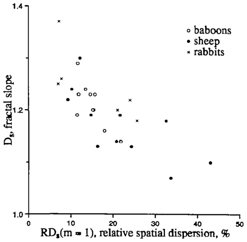
Fractal dimension Ds for spatial variation versus RDs(m=l), the relative dispersion of left ventricular myocardial flows at a voxel size of 1 g.
Discussion
Two points are clarified by this study. First, observed variation in regional myocardial blood flow increases as the resolution is increased, and second, a two parameter fractal relation is a strikingly accurate descriptor of this change that satisfies the need for a summary of the data over the 20-to 40-fold range of sample sizes in our data. The mere fact that two parameters, the dispersion at a particular resolution RD(mref) and a noninteger slope (or fractal dimension Ds), describe the observations over a wide range of observed element sizes is a useful attribute that augments our set of descriptive statistical tools. The two-parameter description is useful for describing the variances in intensities of a characteristic over a domain that has no a priori definition of the unit size, and might augment standard statistical approaches.
The accuracy of the fractal descriptor raises the question of whether there is a true fractal phenomenon underlying the observations of regional flow. A purely deterministic branching network with a constant set of rules (e.g., a constant ratio of parent-to-child branch lengths, constant branch angles, and fixed ratios of diameter to length at each generation) will have the same resistance to flow in all the branches of a given generation and will give uniform flow per unit volume in the supplied regions. Such deterministic rules are unlikely to lead to the situation that we observe in the myocardium: a remarkable nonuniformity of flow. On the other hand, there is no reason that the set of rules need be purely deterministic. Equally valid rules might be that each generation branches with a fixed mean angle plus or minus a prescribed random variation with branch lengths and diameter ratios also fulfilling precisely defined statistical rules. A set of stochastic rules of this type does not lead to uniformity as the different branches of the same generation will now have different resistances, and chance alone will lead to a wide range of flows in the terminal branches. The wider the individual variances prescribed by the rules, the broader will be the heterogeneity of observed regional flows.
The data of Suwa et al15 and Suwa and Takahashi16 show that the renal and mesenteric arteriolar trees have rather consistent log-log relations in ratios of branch lengths, diameter ratios, wall thickness to diameter ratios, radius-to-length ratios, and even intra-arterial pressures over up to a 200-fold range of lengths. These types of data are not yet available for the heart. It will be very worthwhile to undertake detailed studies of the geometry of the myocardial microvasculature and its variability in the intact state. Given sufficient information on the vascular geometry, a “fractal heart” model could be generated. This would require development of a set of rules governing the branching, lengths, diameters, etc. that adheres to the space-filling nature of the system of capillary-tissue units. The data presented in this study can serve as a test of the adequacy of any such model. Other tests would include the vascular resistances, volumes, pressures, and velocities, all of which are observable.
As the spatial resolution for cardiac flow imaging has improved, flow heterogeneity in the normal human myocardium has recently come under consideration. While the resolution of thallium imaging is so low that local variation is not seen in normal hearts, with the higher resolution positron emission tomography (PET)17 the level of variability described in our animal studies can be recognized, but not accurately quantitated, in humans. Such recognition of the normal variation is important in defining the limits of “normality” in more precise terms than has been previously required. One wishes to avoid making diagnoses of regional underperfusion in what are actually normal people. This is especially important as it now appears that early evidence of certain cardiomyopathies may lie in an observation of flow heterogeneity.18 The approach used in these studies to obtain the data on dispersion versus sample size could be applied to PET data. Starting with the highest resolution PET image, adjacent voxels could be combined in an ordered manner to give a set of lower resolution images that could be analyzed for flow heterogeneity. Thus, while the resolution of PET does not approach that of tissue sectioning techniques, the use of the fractal descriptor may allow extrapolation of the PET results down to the level of tissue sectioning resolution if the fractal relation holds to that level. Experiments are needed at much higher resolution to see how far one can go with this idea.
Another application of the knowledge on flow heterogeneity is in the analysis of data on solute exchange. The multiple indicator technique provides a good example. When a set of tracers are injected into the inflow of an organ and a set of outflow dilution curves is obtained by sequential sampling from the outflow, the estimation of kinetic rate constants for membrane permeation or chemical reaction are dependent on the estimates of heterogeneity of flows or transit times through the organ. For example, if the relative dispersion of regional flows is 40%, the myocardial capillary permeability-surface area products for sugars are underestimated by over 50% when the capillary flows are considered uniform instead of accounting for the flow heterogeneity.19 This is a situation where one would like to use the fractal relationship to predict the degree of heterogeneity at the level of the functional microvascular unit size. If the fractal relationship holds down to this unit size, one would predict the heterogeneity by extrapolation and use it in the model analysis of the observed dilution curves. Our linear fractal relationships predict that, if the unit size is of the order of one cubic millimeter, the relative dispersion of flows would be more than 60%. This would give a larger estimate of capillary PS than would be obtained by assuming uniform flow, as much as 80% larger. There are two problems with simply taking the bull by the horns and applying this “fractal fix.” The first is that the actual microvascular unit size is not precisely known; the second is that there is no assurance that the fractal relationship holds down to that level. Important new inferences on the unit size from the observations of Shozawa et al20 suggest a volume of one fifth to one third of a cubic millimeter, smaller than the half to one cubic millimeter that Bassingthwaighte et al21 conjectured. The extension of the fractal relation down to the ultimate unit size is an unlikely event. Rather, one would expect that the relative dispersion of flows would begin to plateau before this limit is reached, because one expects that flows in nearby or adjacent regions to be more similar to each other than are flows in regions distant from each other. This similarity is in keeping with our results showing a fractal dimension of about 1.2 in these hearts, whereas a purely random process would have a fractal dimension of 1.5. The association of flows in neighboring regions demands further study with techniques providing data of very high resolution.
Structures of a uniform grain size can show up as peaks in the fractal plot, as illustrated and analyzed by Wright and Karlsson.6 They show that when there is variation in the grain sizes the peaks are less distinct. In our plots, there is no evidence of peaks deviating from a fractal line. This could conceivably mean that our sequence of steps between the piece masses used was simply so coarse that a peak was missed. If that were so, one might have expected to find a hint of a peak, a point above the fractal line, on at least one animal, but none was seen. The likely explanation is that there is no fundamental grain size or functional unit size above the size of the terminal vascular unit and which is much smaller than our crude piecing can reveal.
This study provides no insight into whether or not the regional flows are related to local metabolic needs. Certainly some variation in local metabolism is expected, as the fractions of connective tissue, myocytes, etc., must vary somewhat. The natural expectation is that metabolism drives local flow. While flow and metabolism must be fairly closely related in a functioning organ, it may also be that the branching of the vascular tree leads inevitably to flow heterogeneity that influences the growth and development of the local capacity for metabolism.
Fractal relations describe the degree of flow heterogeneity over a wide range of sample volumes in the hearts of baboons, sheep, and rabbits. Further studies are needed to elaborate the generality of these findings and to define the limits of applicability of the concept. The relation is not yet based in a secure way on the nature of the vascular tree or its dynamic behavior, although there are reasonable inferences that this may be so. How far this concept extends toward the functional microvascular units where the exchange occurs is unknown, but among the incentives to discover how far the idea can be carried is the need to account for flow heterogeneity when making estimates of transport rates, membrane permeabilities, and intracellular reaction rates in vivo, all of which are needed for both physiological studies and for the interpretation of images obtained in clinical situations by positron and single photon emission tomography.
Acknowledgments
The authors are grateful for the assistance of Alice Kelly in the preparation of the manuscript.
Supported by grants HL-19135, HL-38736, and RR-01243 from the National Institutes of Health.
Appendix: Fractal Dispersions of Densities
This appendix provides numerical examples of aggregates of randomly varying values. The purpose is to illustrate that the fractal dimension is lower for correlated than for random phenomena.
Begin with observations in a spatial domain of the intensities of a property. Examples are the number of stars or galaxies per unit volume in space, the number of cape buffalo per hectare in the Serengeti, or the specific gravity of a milliliter of angel cake. Even though the measurement is error free, there is variation in each concentration or density, just as there is for regional blood flows in the heart. The coefficient of variation, the RD, is an index of the variability or heterogeneity within the domain. If the variation is perfectly random, then any one set of observations at a particular size of observed unit serves to characterize it completely. The reason this can be claimed as a complete characterization is that no matter how the samples are grouped, the standard deviation of a set of aggregates of random values is predictable from the size of the aggregate, Magg, compared with any other aggregate size, Maggo; thelarger the sizes of the aggregates, the smaller the variation amongst aggregates of the particular size:
By aggregating nearest neighbors, the variance decreases. When the individual values of the smallest elements are purely random Gaussian, and no ordering of the array has been undertaken, then the fractal D is 1.5 and a doubling of the size of the aggregate reduces the variance by 30% or the SD to 1/2:
Even when the statistical basis is weak, by virtue of using only small numbers, this works pretty well, as shown in Figure A.1, and the slope gives a fractal D of nearly 1.5. Note that the observed SD at _N_=4, where the 256 values form aggregates of 64 values each, is less than the expected value of 50/8 or 6.25%; the hearts show this same tendency.
Figure A.1.

Two examples of the fractal behavior of the two sets of 256 Gaussian random numbers with mean = 1.0 and SD=50% grouped together by 2s to form 128 aggregates, by 4s to form 64 aggregates, etc The theoretical fractal D is 1.5. Even with such poor statistics, especially for the large aggregates where the number of aggregates (N) is small (32, 16, and 8), the recursive grouping of nearest neighbors results in an observed log-log regression line with a fractal D close to the theoretical value of 1.5.
There is no law that says that log RD versus log N for the pieces of the heart or for the number of aggregates of nonrandom numbers should show self-similarity on recursion, which is what a straight line indicates. However, the grouping of neighbors must give a monotonically decreasing RD. To exemplify a couple of the possibilities of what would be the result of using the same approach on nonrandom arrays of numbers, we created ordered arrays out of random arrays. We have not yet devised a general approach to this and therefore chose to test our procedures on highly coordinated arrays created by exact rank ordering within groups. Rank ordering gives the highest degree of correlation between nearest neighbors in a group, and will serve to illustrate that such ordering creates results which are very different from the fractal relation.
Figure A.2 shows an example of the effects of rank ordering of densities or numbers from a Gaussian distribution with mean 1.0 and standard deviation 0.30. Beginning with an array of 220 random Gaussian numbers, recursive twofold aggregating of neighbors gives successive reductions of RD; the result is the straight line labeled D=1.5. This is the line predicted by theory and illustrates the same phenomenon as in Figure A.1, except that now using large numbers gives a closer approximation to the theory. The straight line is in accord with self-similarity, that is, the reduction in apparent dispersion is the same with each doubling of aggregate size. Randomizing phenomena such as diffusion fit this scheme.
Figure A.2.

Relative dispersion as a function of number of nearest-neighbor aggregates for a randomly ordered and three partially rank-ordered arrays of 220 random numbers with mean 1.0 and SD=0.30. The “cuts” into the array to form the aggregates begin at the first number.
Three other analyses were done by aggregating nearest neighbors after rank ordering subsets of the 220 random numbers. The rank ordering was done by taking Ng points (with Ng=256; 1,024; or 16,384 points in a group) and putting the smallest value in the group first, the next higher value next, and so on up to the highest value in the group last. Then a plot of the 220 points in order would appear as a sawtooth function with monotonic rises along each tooth and some variability in the tooth shape and height. The sequences of 220 points if plotted as value versus index now forms a rough sawtooth; Ng×N=220 so that, with Ng=256 there are 212 teeth, each a rough ramp; with Ng=210 there are 210 teeth and with Ng=214(=16,384) there are 64 teeth. After this within-group rank ordering, the recursive nearest neighbor aggregation gives quite a different shape of RD versus group size. Because of the rank ordering, nearest neighbors in the array are closely similar, so there is very little reduction in the overall dispersion, that is, RD is reduced very little initially by the successive pairings as one progresses from the rightmost point on the graph (unpaired 220 observations) to successively larger groups.
However, as the successive pairings, from right to left, increase the group size toward that of the rank ordered groups (the teeth), the RD diminishes rapidly within a few successive pairings. For Figure A.2, the successive pairings were done by starting with the first of 220 numbers, so that when the number in a group exactly matched the number in a rank-ordered “tooth,” the RD matches the theoretical value for a random array. This is as it should be for the content of the group of the size of the “tooth” or larger is exactly the same whether or not it had been rank-ordered internally.
Consider flows in the heart to be truly random but ordered within small regions. This approach is analogous to considering the heart to be composed of N independent regions into which flow is delivered by an artery of size A, which in turn bifurcates into 220–N or 2N separate but ordered microvascular units. When the heart is divided into samples or groups of units smaller than that supplied by one artery of size A, then the apparent relative dispersion is close to that of a whole population of 220 units. When the heart is divided exactly along borders between the 2N groups supplied by arteries of size A or into larger groups, the RD appears as if the system were random, which it is in this case at the larger sample masses.
Next, consider the same situation as in Figure A.2, but make only a small change, namely the point in the array where the sampling is started, the first cut made. Instead of starting with the first of the 220 values, we started at a random point and cycled through the 220 values (going to the last, then to first and up to the one before the starting point). The result is considerably different from that in Figure A.2, as shown by the curves in Figure A.3. Firstly, as one pairs nearest neighbors successively into larger and larger aggregates of size Ng, the diminution in RD, down from 0.3 is more rapid than in Figure A.2. This refers to the slopes near the right top end of each curve. The second difference is in the apparent RD at N=M, that is, where the number of groups equals the number of rank-ordered “teeth”; the RD is about 1/2 or less than the pure random expectation. At smaller N, larger aggregates, the RDs diminishing thereafter with a fractal slope D<1.5, about D=1.33. (The calculation for D from any pair of points on the graph is Equation 7 of the text.)
Figure A.3.

Relative dispersion as a function of number of nearest-neighbor aggregates for a randomly ordered and three partially rank-ordered, arrays of 220 random numbers with mean 1.0 and SD=0.30. The “cuts” into the array to form the aggregates begin at a random number.
Having a random starting point for the 220 points is like having an arbitrary starting point for slicing up the heart and cutting it without any specified relation to the cognate beds of the supplying arteries. For the random numbers, starting randomly within ordered groups, giving a D of 1.33 means that the RD doubles in three slicings into halves (2→8 pieces) whereas purely random unordered arrays double their apparent RD with two slicings (2→4 pieces). Perhaps we can extrapolate from this to suggest that if in the heart our slicing patterns fail to match the cognate beds of individual arteries, there will be some reduction in the apparent Ds compared with that obtainable with slicing at the peripheries of individual regions.
The parts of Figures A.2 and A.3 which are probably most relevant to our experimental observations are the regions with RDs greater than 10%. For each rank-ordered group size, when increasing N, as soon as N exceeds 220/Ng, the lines of RD versus aggregate size show curves quickly reaching the plateau at 30%. These are quite unlike our data. Rank-ordering of the values within the group gives maximal local correlation; thus our local rank ordering of random values is a poor analogue to the physiological situation. The data lie in the region encompassed above by rank-ordering of large groups of random numbers (too near the plateau, too curved, flatten too fast with increasing division) and the unsorted random values (too low RDs for large samples and too steep a slope). We have no algorithm for the intermediate situation that might match the data, but we can be confident that it is very different from purely random flows and very different from groups with closely correlated rank ordered flows. From the Dss observed in the heart we expect nearest neighbor correlations of _r_=23–2D − 1 or about 0.5. We recognize that the random number string is a one-dimensional representation whereas the myocardial flows are distributed three dimensionally. Local correlation in three dimensions is to be expected, and it is probably necessary to account for the distributions in much more detail in order to understand our observations. The approach suggested by Voss22 considering the values at partially correlated noise will certainly be useful. While we don’t know its basis in vascular anatomy, rheology, and local regulation of regional flows, the fractal relations provide a fascinating new descriptive approach to sorting out the problem.
References
- 1.Yipintsoi T, Dobbs WA, Jr, Scanlon PD, Knopp TJ, Bassingthwaighte JB. Regional distribution of diffusible tracers and carbonized microspheres in the left ventricle of isolated dog hearts. Circ Res. 1973;33:573–587. doi: 10.1161/01.res.33.5.573. [DOI] [PMC free article] [PubMed] [Google Scholar]
- 2.King RB, Bassingthwaighte JB, Hales JRS, Rowell LB. Stability of heterogeneity of myocardial blood flow in normal awake baboons. Circ Res. 1985;57:285–295. doi: 10.1161/01.res.57.2.285. [DOI] [PMC free article] [PubMed] [Google Scholar]
- 3.Bassingthwaighte JB, Malone MA, Moffett TC, King RB, Little SE, Link JM, Krohn KA. Validity of microsphere depositions for regional myocardial flows. Am J Physiol. 1987;253 doi: 10.1152/ajpheart.1987.253.1.H184. [DOI] [PMC free article] [PubMed] [Google Scholar]; Heart Circ Physiol. 22:H184–H193. [Google Scholar]
- 4.Yen RT, Fung YC. Effect of velocity distribution on red cell distribution in capillary blood vessels. Am J Physiol. 1978;235 doi: 10.1152/ajpheart.1978.235.2.H251. [DOI] [PubMed] [Google Scholar]; Heart Circ Physiol. 4:H251–H257. doi: 10.1152/ajpheart.00206.2004. [DOI] [PubMed] [Google Scholar]
- 5.Marcus ML, Kerber RE, Erhardt JC, Falsetti HL, Davis DM, Abboud FM. Spatial and temporal heterogeneity of left ventricular perfusion in awake dogs. Am Heart J. 1977;94:748–754. doi: 10.1016/s0002-8703(77)80216-0. [DOI] [PubMed] [Google Scholar]
- 6.Wright K, Karlsson B. Fractal analysis and stereological evaluation of microstructures. J Microsc. 1983;129:185–200. [Google Scholar]
- 7.Bassingthwaighte JB, van Beck JHGM. Lightning and the heart: Fractal behavior in cardiac function. Proc IEEE. 1988;76:693–699. doi: 10.1109/5.4458. [DOI] [PMC free article] [PubMed] [Google Scholar]
- 8.Peitgen HO, Saupe D, editors. The Science of Fractal Images. New York: Springer-Verlag, New York, Inc; 1988. [Google Scholar]
- 9.Mandelbrot B. Fractals: Form, chance and dimension. San Francisco: WH Freeman & Co; 1977. [Google Scholar]
- 10.Mandelbrot BB. The fractal geometry of nature. San Francisco: WH Freeman & Co; 1983. [Google Scholar]
- 11.Heymann MA, Payne BD, Hoffman JIE, Rudolph AM. Blood flow measurements with radionuclide-labeled particles. Prog Cardiovasc Dis. 1977;20:55–79. doi: 10.1016/s0033-0620(77)80005-4. [DOI] [PubMed] [Google Scholar]
- 12.Bassingthwaighte JB, Malone MA, Moffett TC, King RB, Chan IS, Link JM, Krohn KA. Molecular and particulate depositions for regional myocardial flows in sheep. Circ Res. doi: 10.1161/01.res.66.5.1328. (in press) [DOI] [PMC free article] [PubMed] [Google Scholar]
- 13.Berkson J. Are there two regressions? J Am Stat Assoc. 1950;45:164–180. [Google Scholar]
- 14.Utley J, Carlson EL, Hoffman JIE, Martinez HM, Buckberg GD. Total and regional myocardial blood flow measurements with 25μ, 15μ, 9μ, and filtered l–10μ diameter microspheres and antipyrine in dogs and sheep. Circ Res. 1974;34:391–405. doi: 10.1161/01.res.34.3.391. [DOI] [PubMed] [Google Scholar]
- 15.Suwa N, Niwa T, Fukasawa H, Sasaki Y. Estimation of intravascular blood pressure gradient by mathematical analysis of arterial casts. Tohoku J Exp Med. 1963;79:168–198. doi: 10.1620/tjem.79.168. [DOI] [PubMed] [Google Scholar]
- 16.Suwa N, Takahashi T. Morphological and morphometrical analysis of circulation in hypertension and ischemic kidney. Munich: Urban & Schwarzenberg; 1971. [Google Scholar]
- 17.Budinger TF, Huesman RH. Ten precepts for quantitative data acquisition and analysis. Cardiovascular Metabolic Imaging: Physiological and Biochemical Dynamics in vivo. In: McMillin-Wood JB, Bassingthwaighte JB, editors. Circulation. suppl IV. Vol. 72. 1985. pp. 53–62. [PubMed] [Google Scholar]
- 18.Eng C, Cho S, Factor SM, Sonnenblick EH, Kirk ES. Myocardial micronecrosis produced by microsphere embolization: Role of an α-adrenergic tonic influence on the coronary microcirculation. Circ Res. 1984;54:74–82. doi: 10.1161/01.res.54.1.74. [DOI] [PubMed] [Google Scholar]
- 19.Bassingthwaighte JB, Goresky CA. Modeling in the analysis of solute and water exchange in the microvasculature. In: Renkin EM, Michel CC, editors. Handbook of Physiology, Section 2: The Cardiovascular System, Volume IV, Microcirculation, Chapter 13. Bethesda, Md: American Physiological Society; 1984. pp. 549–626. [Google Scholar]
- 20.Shozawa T, Kawamura K, Okada E. Study of intramyocardial microangioarchitecture with respect to pathogenesis of focal myocardial necrosis. Bibl Anat. 1981;20:511–516. [Google Scholar]
- 21.Bassingthwaighte JB, Yipintsoi T, Harvey RB. Microvasculature of the dog left ventricular myocardium. Microvasc Res. 1974;7:229–249. doi: 10.1016/0026-2862(74)90008-9. [DOI] [PMC free article] [PubMed] [Google Scholar]
- 22.Voss RF. Fractals in nature: From characterization to simulation. In: Peitgen HO, Saupe D, editors. The Science of Fractal Images. New York: Springer-Verlag New York, Inc; 1988. pp. 21–70. [Google Scholar]