nFuse: Discovery of complex genomic rearrangements in cancer using high-throughput sequencing (original) (raw)
Abstract
Complex genomic rearrangements (CGRs) are emerging as a new feature of cancer genomes. CGRs are characterized by multiple genomic breakpoints and thus have the potential to simultaneously affect multiple genes, fusing some genes and interrupting other genes. Analysis of high-throughput whole-genome shotgun sequencing (WGSS) is beginning to facilitate the discovery and characterization of CGRs, but further development of computational methods is required. We have developed an algorithmic method for identifying CGRs in WGSS data based on shortest alternating paths in breakpoint graphs. Aiming for a method with the highest possible sensitivity, we use breakpoint graphs built from all WGSS data, including sequences with ambiguous genomic origin. Since the majority of cell function is encoded by the transcriptome, we target our search to find CGRs that underlie fusion transcripts predicted from matched high-throughput cDNA sequencing (RNA-seq). We have applied our method, nFuse, to the discovery of CGRs in publicly available data from the well-studied breast cancer cell line HCC1954 and primary prostate tumor sample 963. We first establish the sensitivity and specificity of the nFuse breakpoint prediction and scoring method using breakpoints previously discovered in HCC1954. We then validate five out of six CGRs in HCC1954 and two out of two CGRs in 963. We show examples of gene fusions that would be difficult to discover using methods that do not account for the existence of CGRs, including one important event that was missed in a previous study of the HCC1954 genome. Finally, we illustrate how CGRs may be used to infer the gene expression history of a tumor.
Cancer is a genomic disease characterized by unregulated cell growth resulting from acquired or inherited DNA changes. Genome rearrangements are an important class of DNA changes, known to disrupt the activity of tumor suppressor genes and promote increased activity of oncogenes. Genome rearrangements are also known to create fusion genes: Novel oncogenes formed when a rearrangement juxtaposes two or more existing genes. Fusion genes are the defining molecular feature of many cancers and represent potential drug targets in those cancers. A classic example is the _BCR_-ABL1 gene fusion present in 95% of chronic myelogenous leukemia patients and targeted by the drug iminitib.
The molecular mechanisms that cause somatic genome rearrangements are still the focus of investigation. Double-stranded DNA breaks followed by a ‘joining event’ are known to result in a simple genomic rearrangement consisting of a single breakpoint, where a breakpoint is defined as a pair of genomic locations that are distant in the normal genome but adjacent in the tumor genome. A breakpoint can be considered as the most basic unit of rearrangement. Examples of processes that generate single breakpoints include nonhomologous end joining, homologous recombination-mediated repair, and a single cycle of breakage-fusion-bridge (Bignell et al. 2007).
Recently discovered are complex genomic rearrangements (CGRs), rearrangements composed of multiple breakpoints with a specific structure. In prostate cancer, for example, Berger et al. (2011) discovered closed chains of breakage and rejoining (CCBRs). Berger et al. (2011) suggested that a CCBR potentially occurs when distant chromosomal regions are spatially colocalized in the nucleus, possibly because they have been recruited by the same transcriptional factory. Importantly, they showed that biologically relevant gene fusions, such as TMPRSS2-ERG, were created by CCBR events. CCBRs are balanced rearrangements: They result in little or no loss of genomic material. It has been proposed that balanced rearrangements are more likely to produce functional gene fusions (Mitelman et al. 2007).
Other cancers exhibit an entirely different type of CGR produced by a shattering of chromosomal regions, followed by a reassembly from the resulting fragments (Stephens et al. 2011). As a result, some breakpoints between large chromosomal segments contain additional smaller fragments (genomic shards) interposed at the breakpoint (Bignell et al. 2007). These genomic shards originate from other regions affected by the catastrophe, typically at the boundaries of deleted regions (Bignell et al. 2007). Breakpoints with small (∼500-bp) genomic shards interposed at the breakpoint are termed complex and have been identified previously in breast cancer (Stephens et al. 2009). Breakpoints with larger fragments of other genes interposed at the breakpoint have the potential to create polyfusions (Wu et al. 2012a), fusion genes composed of three or more separate genes. Both complex breakpoints and polyfusions are rearrangements composed of two or more simple breakpoints, and identification of all breakpoints is required to discover the fusion.
High-throughput paired-end whole-genome shotgun sequencing (WGSS) is currently the most efficient method of identifying breakpoints in tumor genomes. Briefly, WGSS can be used to sequence the ends of short fragments of DNA produced by fragmentation of a tumor genome. The pairs of end sequences (paired-end reads, or simply reads) can then be mapped back to a healthy reference genome sequence. Distantly mapping reads or reads that map with unexpected orientation can then be used to predict breakpoints. WGSS, however, presents many unique challenges compared with earlier technologies. The presence of repeated regions in the genome and short WGSS read lengths complicate the problem of unambiguously identifying the origin of some WGSS reads. Furthermore, sequencing errors lead to some proportion of false reads. Both of these problems are magnified due to the huge size of WGSS data sets. Finally, aneuploidy, tumor heterogeneity, and cellularity have the combined effect of diluting the sequence signal of breakpoints, even in high coverage WGSS data sets. Nevertheless, solutions now exist for accurately predicting breakpoints from WGSS (Chen et al. 2009; Hormozdiari et al. 2009, 2011; McPherson et al. 2011b; Wang et al. 2011), though a true account of false-negative rates remains elusive.
Given the ability to predict breakpoints in WGSS, an important question is how to infer genome structure from these breakpoints, and potentially reconstruct chromosomal architectures. In a recent study, Greenman et al. (2011) propose methods for reconstructing ‘digital karyotypes’ from copy number and breakpoint predictions. Their method requires precise breakpoint predictions and could not guarantee a unique solution for a reasonably complex genome. Previous to Greenman et al. (2011), efforts to reconstruct tumor genomes relied on low resolution data such as fluorescence in situ hybridization (FISH) and bacterial artificial chromosome (BAC) sequencing (Raphael et al. 2003; Raphael and Pevzner 2004; Ozery-Flato and Shamir 2009). These methods may be sufficiently sensitive to reconstruct large-scale rearrangements; however, they will likely miss complex focal rearrangements.
In this study, we propose a method for reconstructing CGRs from WGSS data. Crucial to the problem of identifying CGRs is the missing data problem: identification of a CGR relies on the identification of all n breakpoints in the CGR. Therefore, the basis for our approach is a high sensitivity method for predicting breakpoints. However, WGSS read alignment data contains a significant amount of noise, and this noise will produce false-positive predictions, especially with a method that prioritizes sensitivity. Thus we calculate a probability for each breakpoint that reflects our belief in its existence. Like the aforementioned studies, we identify CGRs using breakpoint graphs (Pevzner 2000). We incorporate the breakpoint probability into the graph, and use that probability to guide our search for high probability structures representing potential CGRs. We prioritize our search for CGRs based on fusion transcript predictions from matched high-throughput cDNA sequencing (RNA-seq), thereby using effect on the transcriptome as an indicator of potential functional significance.
We have applied our method, nFuse, to publicly available WGSS and RNA-seq data for the well-characterized breast cancer cell line HCC1954. We show that we are able to rediscover a significant proportion of previously discovered breakpoints. Furthermore, we show that the breakpoint probability we calculate accurately separates the previously discovered breakpoints from a background of predominantly false-positive predictions. By use of long-range PCR (LR-PCR), we validated five out of six polyfusions predicted by nFuse for HCC1954. We have also applied nFuse to WGSS and RNA-seq data generated from primary human prostate cancer sample 963 (Wu et al. 2012b). By use of a CCBR discovered in 963, we illustrate how CCBRs can be used to infer the gene expression history of a tumor. Finally, we present an example of a CCBR with a complex breakpoint discovered in 963, providing a link between CCBR and complex breakpoints.
Methods
Complex rearrangement discovery using breakpoint graphs
Complex rearrangements involve two or more breakpoints, such that the set of breakpoints elicit a specific structure. To identify complex rearrangements, we employ a construct called the breakpoint graph (Pevzner 2000). The complex rearrangements we are interested in discovering naturally arise as features of the breakpoint graph. Unlike previous breakpoint graph approaches, the breakpoint graph we construct includes a measure of the uncertainty inherent in breakpoint predictions produced from WGSS data. Our algorithms then seek to identify CGRs more likely to be real by searching for the higher probability structures in the breakpoint graph.
Of crucial importance is the effect of missing data on our ability to predict CGRs. For a CGR composed of n breakpoints, failing to predict any one of those n breakpoints will result in a failure to identify the CGR. To mitigate this problem, we seek to include in the breakpoint graph all reasonable breakpoint predictions, including those nominated by reads with ambiguous genomic origin. Thus the breakpoint graph we construct will contain a large amount of noise, and the majority of breakpoints are expected to be false positives. A real but low probability breakpoint may then be identified as part of a CGR, providing the probabilities of the CGR's other breakpoints are sufficiently high. In contrast, removing low probability breakpoints before building the breakpoint graph would also remove the aforementioned real breakpoint, making it impossible to identify the CGR.
nFuse seeks to identify two types of CGRs: CCBRs (Berger et al. 2011) and polyfusions/complex breakpoints. We emphasize here that these two types of CGRs are very different types of events, unified by breakpoint graphs as a common computational representation. We introduce the concept of the breakpoint graph by first focusing on polyfusions and complex breakpoints, after which we describe CCBRs and their breakpoint graph representation.
Breakpoint graph structure
A breakpoint is an adjacency in one genome that does not exist in another genome. In the context of cancer genomics, we are interested in identifying adjacencies in the tumor genome not found in the normal (or reference) genome. Such unexpected adjacencies are evidence of somatic rearrangement and may have important implications for tumor biology. For instance, an unexpected adjacency between the 5′ exons of gene A and the 3′ exons of gene B may represent an A-B fusion gene that drives proliferation of a tumor.
The breakpoint graph is a representation of a set of unexpected adjacencies, or breakpoints. We use the breakpoint graph to represent the set of breakpoints identified in a tumor genome that are not in the reference genome. The graph is defined on a set of vertices representing the set of nucleotides that are adjacent in the reference but not in the tumor. The graph contains two types of edges, breakpoint edges and adjacency edges. Breakpoint edges represent adjacencies in the tumor, while adjacency edges represent a putatively contiguous region of the reference genome not interrupted by a breakpoint. Note that for identification of CCBRs, we generalize adjacency edges as described in the CCBR section below.
Consider the following example illustrated in Figure 1. Let _A_1 and _A_2 be adjacent nucleotides in reference chromosome A and let _B_1 and _B_2 be adjacent nucleotides in reference chromosome B and suppose we identify an _A_1, _B_2 breakpoint (Fig. 1A). The graph for the _A_1, _B_2 breakpoint contains vertices for _A_1, _A_2, _B_1, and _B_2, in addition to the breakpoint edge (_A_1, _B_2) (Fig. 1B). Now consider an additional _B_3, _C_1 breakpoint between chromosomes B and C (Fig. 1C). In addition to the (_B_3, _C_1) breakpoint edge, the graph also contains a (_B_2, _B_3) adjacency edge representing a putatively contiguous region in the tumor between nucleotides _B_2 and _B_3 (Fig. 1D). Finally consider a fourth breakpoint between chromosomes A and B (Fig. 1E) represented by an (_A_3, _B_5) breakpoint edge (Fig. 1F). The breakpoint graph will also contain a (_B_2, _B_5) adjacency edge representing the possibility that the (_B_3, _C_1) does not exist in a putative tumor chromosome that contains both the (_A_1, _B_2) and (_B_5, _A_3) breakpoints. Thus each breakpoint will be considered optional in our realization of the breakpoint graph. To reflect this, we define adjacency edges as follows. Let _X_left, _X_right be a pair of nucleotides adjacent in the reference with a breakpoint edge incident on _X_left. We add an adjacency edge from _X_left to every upstream right vertex. Similarly, if a breakpoint edge is incident on _X_right, we add an adjacency edge from _X_right to every downstream left vertex.
Figure 1.

Breakpoint graphs and polyfusions. (A) A breakpoint as an unexpected adjacency. (B) The breakpoint graph for a single breakpoint showing a breakpoint edge. (C) Two breakpoints on chromosomes A, B, and C. (D) The breakpoint graph for the two breakpoints showing two breakpoint edges and an adjacency edge. (E) Three breakpoints on chromosomes A, B, and C. (F) The breakpoint graph for the three breakpoints showing a (_B_2, _B_5) adjacency edge that encodes the optional nature of breakpoint (_B_3, _C_1). (G) Breakpoints for an X-Y gene fusion with a complex breakpoint. (H) The breakpoint graph for the complex breakpoint showing an alternating path between X and Y.
Polyfusions and complex breakpoints
A key feature of the breakpoint graph is that every alternating path represents a putative tumor chromosome. Polyfusions and complex breakpoints are subsequences of tumor chromosomes and as such will be represented as alternating paths given successful identification of all relevant breakpoints. As an example, consider a fusion between gene X on chromosome A and gene Y on chromosome C, for which a fragment of chromosome B is interposed at the breakpoint (Fig. 1G). In the breakpoint graph, the complex breakpoint will be represented as an alternating path of length 5 between vertices representing the 5′ end of gene X and the 3′ end of gene Y (Fig. 1H). In general, a polyfusion or complex breakpoint involving n loci will be represented in the breakpoint graph as an alternating path of length 2_n_ − 1.
Closed chains of breakage and rejoining
CCBRs can be thought of as a generalization of a reciprocal translocation to n > 2 loci. For a reciprocal translocation, two loci are broken and the broken ends are swapped and rejoined. A three-loci CCBR involves the breakage, permutation, and rejoining of three loci. An example three-loci CCBR event would be the transformation of chromosomes A, B, and C into tumor chromosomes _A_-B, _B_-C, and _C_-A (Fig. 2A).
Figure 2.

Closed chains of breakage and rejoining (CCBRs). (A) In an idealized version of a CCBR, no chromosomal material is lost or gained. (B) Actual CCBRs may involve small loss or gain of chromosomal material. For instance, the _A_2→_A_3 and _C_2→_C_3 sections of chromosomes A and C appear to have been lost, and the _B_2→_B_3 section of chromosome B appears to have been duplicated. (C) The breakpoint graph for the CCBR in B showing (_A_1, _A_4) and (_C_1, _C_4) loss edges and a (_B_2, _B_3) gain edge.
In the ideal case, no chromosomal material will be lost in the exchange (Fig. 2A). As shown in this work and previously (Berger et al. 2011), many instances of chromosomal breakage and rejoining involve the loss or gain of chromosomal material. As a result, the breakpoints at broken and rejoined loci may be separated by an unknown distance. Figure 2B depicts a more realistic example involving chromosomes A, B, and C. In this example, the CCBR has resulted in a loss of small sections of chromosomes A and C. In addition, the _A_-B and _B_-C tumor chromosomes created by the CCBR both include copies of a segment of chromosome B, resulting in a gain of that segment. Of crucial importance, any loss or gain caused by a CCBR will not necessarily be represented by additional breakpoints in the breakpoint graph. Nevertheless, the breakpoint graph, properly defined, will yield CCBRs as a specific type of subgraph.
To identify CCBRs, we augment the previously defined breakpoint graph with additional edges. Call the previously defined adjacency edges as gain adjacency edges. Define additional adjacency edges called loss adjacency edges as follows. Let _X_left, _X_right be a pair of nucleotides adjacent in the reference with a breakpoint edge incident on _X_left. Add loss adjacency edges from _X_left to every downstream right vertex. Similarly, if a breakpoint edge is incident on _X_right, add loss adjacency edges from X_right to every upstream left vertex. A n-loci CCBR in the resulting graph will be represented by an alternating cycle of length 2_n. Figure 2C shows the breakpoint graph for the CCBR in Figure 2B. The breakpoint edges, loss edges (_A_1, _A_4) and (_C_1, _C_4), and gain edge (_B_2, _B_3) together form an alternating six-cycle. Note that an alternative explanation for the breakpoints in Figure 2B is a reciprocal translocation between chromosomes A and C, with a complex breakpoint for the _A_-C chromosome involving a shard of chromosome B. We will explore this ambiguity further when discussing the results for tumor sample 963.
Identifying high-probability CGRs
A breakpoint graph constructed from WGSS data will contain many alternating paths connecting candidate fused genes, and many alternating cycles. Some of the ambiguity arises because the WGSS data are produced from a diploid, or potentially poly-ploid, genome. Tumor chromosomes reassembled from copies of the same reference chromosomes will each produce a set of breakpoints. The WGSS data for these tumor chromosomes will then yield a merged set of all breakpoints. Only in very simplistic instances will it be possible to repartition the merged breakpoints into sets of breakpoints each produced by the same tumor chromosome. Furthermore, the breakpoints obtained from WGSS data will include a significant number of spurious predictions, especially when prioritizing sensitivity as proposed by nFuse. Spurious breakpoint predictions will further increase the number of alternating paths and cycles.
nFuse uses an objective function to identify real CGRs from the background of incidental and false-positive structures. Our objective function is probabilistically motivated and incorporates the probability that each breakpoint exists (breakpoint probability), in addition to a probability calculated for the total length of adjacency edges in the structure (CGR length probability). Inclusion of the breakpoint probability will allow nFuse to mitigate the effects of spurious breakpoint predictions. We model the CGR length probability as an exponential distribution with the scale parameter β and motivate the choice of exponential independently for complex breakpoints/polyfusions and CCBRs in the following sections. The negative log probability of a CGR with breakpoints X and adjacency edge lengths Y can be calculated as given in Equation 1, herein referred to as the CGR score:

Let G be a breakpoint graph with breakpoint edges given distance −log_P_(x) and adjacency edges given distance  . By inspection of Equation 1, an alternating cycle or path that maximizes P(X, Y) will be a shortest alternating cycle or path on G.
Breakpoint prediction and probability estimation
We predict breakpoints from discordant paired end alignments. Our approach aims for high sensitivity by including reads with multiple genomic mappings, and reads that map only partially to the genome. To ensure adequate specificity, we calculate a probability for each breakpoint based on the alignment evidence and use that probability in downstream analysis including CGR discovery.
Let R be the set of paired end WGSS reads. We generate a set of mapping locations M for R using the following well-established strategy (Volik et al. 2003; Tuzun et al. 2005). For each paired end read 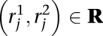 :
:
- Identify a single concordant mapping location if it exists.
- If no concordant mapping location exists:
- a. Identify the n top scoring mapping locations for
 .
. - b. Identify the n top scoring mapping locations for
 .
.
- a. Identify the n top scoring mapping locations for
We identify the n top scoring mapping locations for  (and
(and  ) as follows. Let sj be the maximum alignment score attained by partial alignment of read j to the genome. Briefly, a partial alignment is an alignment of the first ℓ nucleotides of the read, for ℓ that maximizes an alignment score (Supplemental Methods). Let k be the number of mappings of read j that attain sj. If k > n assume the read is unmappable and filter it, otherwise retain the k mapping locations. The study described herein used Bowtie 2 (Langmead and Salzberg 2012) in local alignment mode to obtain partial alignments. We are currently exploring the tradeoff among speed, accuracy, and flexibility of available aligners to allow optimal performance of the nFuse breakpoint prediction.
Let mj ∈ M be the mapping locations identified for read  . Define the following indicator variables:
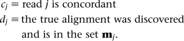
We make the assumption that reads mapped concordantly by the aligner are in fact concordant (with probability 1). We filter the concordantly mapped reads to create the set of discordant reads Rd and set of discordant mappings Md. As a result, P(cj = 1, dj = 1) = 0 for the set of filtered reads. We estimate probabilities for the remaining two possibilities for the true alignment of each read:
We estimate P(cj = 1|·) using the maximum concordant alignment score csj. To calculate csj, we align both ends of read j to all mapping locations in the set mj, and set csj to the maximum alignment score identified by this process. We then calculate P(cj = 1|csj) (Supplemental Methods) and use it to approximate P(cj = 1|·). We approximate P(dj = 1|cj = 0,·) as P(dj = 1|cj = 0, asj) where asj is the alignment score for read j (Supplemental Methods).
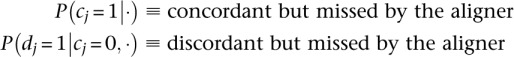
Next, we cluster the discordant alignments Md based on the likelihood that a set of alignments were generated by the same breakpoint (Supplemental Methods). Let the resulting clusters of alignments represent putative breakpoints. Let gij indicate that putative breakpoint i generated read j. Assume gij = 0 if read j is not in the cluster that supports breakpoint i. We estimate P(gij = 1|·) as P(gij = 1|nmj, dj = 1), where nmj is the number of alternate mapping locations of read j. Under the assumption that all mapping locations discovered by the aligner are equally likely, we calculate  .
.
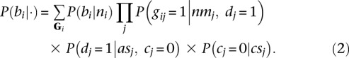
Finally, let bi indicate that breakpoint i is true, let Gi be the set of all gij for breakpoint i, and let ni be the number of reads that were generated by breakpoint i, that is, 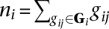 . We estimate P(bi|ni) (Supplemental Methods) and use it to estimate P(bi|·) as given by Equation 2.
Identifying high probability complex breakpoints and polyfusions
Complex breakpoints and polyfusions may be frequently occurring events in a rearranged tumor genome. Without further information, the biological significance of these events will be difficult to quantify. We use fusion transcripts predicted from RNA-seq (McPherson et al. 2011a) to guide our search for complex breakpoints and polyfusions, using effect on the transcriptome as an indicator of potential biological significance. The fusion transcripts also serve as a scaffold for reconstruction of the complex breakpoints/polyfusions.
Given a gene _A_–gene B fusion transcript predicted from RNA-seq, we would like to predict the set of breakpoints that produced the _A_-B fusion. The breakpoints will often occur in the introns of gene A and B. As a result, these breakpoints are often spliced out of the _A_-B fusion transcript. Let xA and xB be the genomic positions of the splice sites in gene A and B that are predicted as spliced together in the fusion transcript. We would like to predict the intron sequence between xA and xB on the tumor chromosome. We model the intron lengths of fusion transcripts using an exponential with rate parameter βp. An alternating path p from xA to xB represents a potential intron for the _A_-B fusion transcript, and the total length of the adjacency edges in p equals the length of the putative intron. Following from the analysis that lead to the CGR score (Equation 1), we reconstruct the most likely intron by searching for the shortest alternating path between xA and xB on the graph G with β = βp. For details on setting βp, see Supplemental Methods.
Identifying high probability CCBRs
Very little is currently known about CCBRs, making model selection difficult. We model the total length of loss and gain adjacency edges in a CCBR using an exponential distribution with rate parameter βc. We selected the exponential because it is the maximum entropy distribution for a positive random variate with fixed mean. For the purposes of this study, we have used βc = 2000 bp. We expect that the future discovery of additional CCBRs will allow us to properly estimate βc.
Similar to complex breakpoints/polyfusions, we search for CCBRs that are associated with fusion transcript predictions. For each breakpoint b associated with a fusion transcript as described in the previous section, we search for a CCBR that includes b. Following from the analysis that lead to the CGR score (Equation 1), we reconstruct the most likely CCBR that includes b by searching G with β = βc for the shortest alternating cycle that includes b. Specifically, we first remove the breakpoint edge (_b_1, _b_2) for breakpoint b from G, then search for the shortest between _b_1 and _b_2.
Results
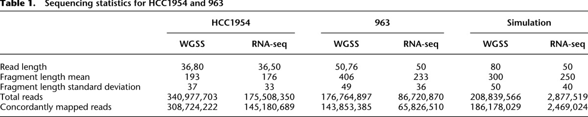
We have used nFuse to identify CGRs in three data sets: a HCC1954 breast cancer cell line data set, a data set derived from primary tumor 963 (Wu et al. 2012b), and a simulated data set that includes 120 synthetic CGRs (for sequencing statistics, see Table 1). We used the HCC1954 data set to assess breakpoint prediction sensitivity and breakpoint scoring specificity and used the simulated data set to assess precision and recall for CGR discovery. CGRs were retained only if their CGR score (Equation 1) was less than 20.
Table 1.
Sequencing statistics for HCC1954 and 963
HCC1954 breast cancer cell line
We first applied our method to publicly available data for HCC1954, a cell line that has been well studied at the molecular level. The HCC1954 cell line was derived from a ductal breast carcinoma and is estrogen receptor negative, progesterone receptor negative, and ERBB2 positive (Zhao et al. 2010). Four recent studies sought to identify rearrangements in HCC1954. Bignell et al. (2007) used end sequencing of BAC libraries to discover rearrangements in tumor amplicons and identified 59 unique breakpoints in HCC1954. Zhao et al. (2009) used long transcriptome reads to nominate fusion transcripts and a combination of LR-PCR and FISH to identify underlying genomic rearrangements. Stephens et al. (2009) used WGSS to discover rearrangements in 24 breast cancers and were able to identify 230 unique breakpoints in HCC1954. Some of the breakpoints discovered by Stephens et al. (2009) were more complex than a breakage and rejoining of two genomic loci. Interposed between the breakpoints were one or more genomic shards: small (<500-bp) fragments of DNA from elsewhere in the genome. Galante et al. (2011) also used WGSS to discover somatic alterations in HCC1954 and identified 77 unique breakpoints. Finally, Asmann et al. (2011) used their pipeline SnowShoes-FTD to identify four fusion transcripts in HCC1954.
We obtained WGSS and RNA-seq data for HCC1954 from the NCBI Sequence Read Archive (SRA; http://www.ncbi.nlm.nih.gov/Traces/sra). The WGSS data (accession no. ERA010917) are the same data used in the study by Galante et al. (2011), and the RNA-seq data (accession no. ERA015355) were produced in a separate study on allele-specific expression (Zhao et al. 2010). Next we compiled a list of 345 validated breakpoints from the studies by Bignell et al. (2007), Stephens et al. (2009), and Galante et al. (2011). Small deletions were excluded from the analysis since they are not the focus of this study. There was very little overlap between the sets of breakpoints discovered in each study, with only three breakpoints common to all three studies.
By use of the previously validated breakpoints, we sought to estimate whether nFuse is sensitive enough to detect a significant proportion of real breakpoints and whether the nFuse breakpoint ranking method could discern between real breakpoints and the background noise of spurious predictions. The breakpoint detection step of the nFuse pipeline identifies 296 of the 345 previously validated true-positive breakpoints, accounting for 91.5% of the Bignell et al. (2007) breakpoints, 81.3% of the Stephens et al. (2009) breakpoints, and 97.4% of the Galante et al. (2011) breakpoints, for a recall of 0.858 (Fig. 3A). In addition to the 296 true-positive breakpoints, nFuse also identifies 2,634,524 additional breakpoints. Since 2,634,524 is well beyond the expected number of breakpoints in a rearranged tumor genome and since we are including even very low probability breakpoint predictions, a large majority of the 2,634,524 are expected to be false positives. We sought to estimate whether the breakpoint probability we calculate could discriminate between true and false breakpoints. We first selected 3000 breakpoint predictions at random and assumed that a significant majority of these predictions were false. Next we compared the scores of the 3000 randomly selected predictions to the scores of the true-positive predictions (Fig. 3B), finding that the true-positive predictions scored significantly better than the randomly selected predictions (P < 2.2 × 10⁻¹⁶ Wilcoxon rank sum test).
Figure 3.

Performance of nFuse breakpoint prediction on breakpoints previously discovered in HCC1954. (A) Shown is the overlap between sets of breakpoints discovered by Bignell et al. (2007), Stephens et al. (2009), Galante et al. (2011), and nFuse. Previously discovered breakpoints are rediscovered by nFuse with a recall of 0.858. (B) Beanplot comparing nFuse breakpoint scores for a random selection of 3000 nFuse breakpoint predictions, and the 296 ‘true positive’ nFuse breakpoint predictions. Score is calculated as −log probability. The nFuse breakpoint scoring ranks true-positive breakpoints significantly higher (closer to zero) than random breakpoints, many of which are expected to be false positives.
Next we used a breakpoint graph constructed from the 2,634,524 HCC1954 breakpoints to predict CGRs in HCC1954 (for summaries of CCBRs and complex breakpoints, respectively, see Tables 2 and 3). We then attempted to validate the top six complex breakpoint/polyfusion predictions as ranked by CGR score (Equation 1). For validation, we performed LR-PCR across the entire length of the complex breakpoint/polyfusion. An event was considered validated if the size of the PCR product matched the predicted length and if Sanger sequencing of both ends of the PCR product matched the predicted sequence. Five out of six LR-PCR assays produced PCR products, four of the predicted size. The PCR product for _PHF20L1_-SAMD12 was ∼1.5 kbp longer than expected. We confirmed by PCR that each of the three individual breakpoints predicted to form the _PHF20L1_-SAMD12 polyfusion were present in the _PHF20L1_-SAMD12 PCR product. Thus we conclude that the _PHF20L1_-SAMD12 prediction is correct but potentially incomplete, and we suspect the existence of an additional insertion that is not identified when searching for the least complex solution. The five validated events are shown in Figure 4.
Table 2.
Summary of putative CCBRs discovered in HCC1954
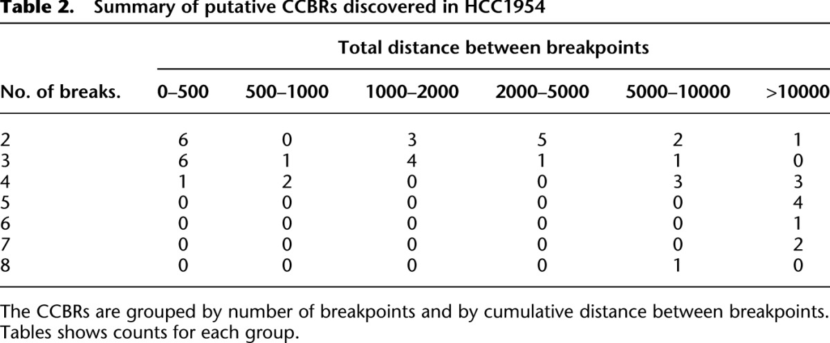
Table 3.
Summary of putative complex breakpoints discovered in HCC1954
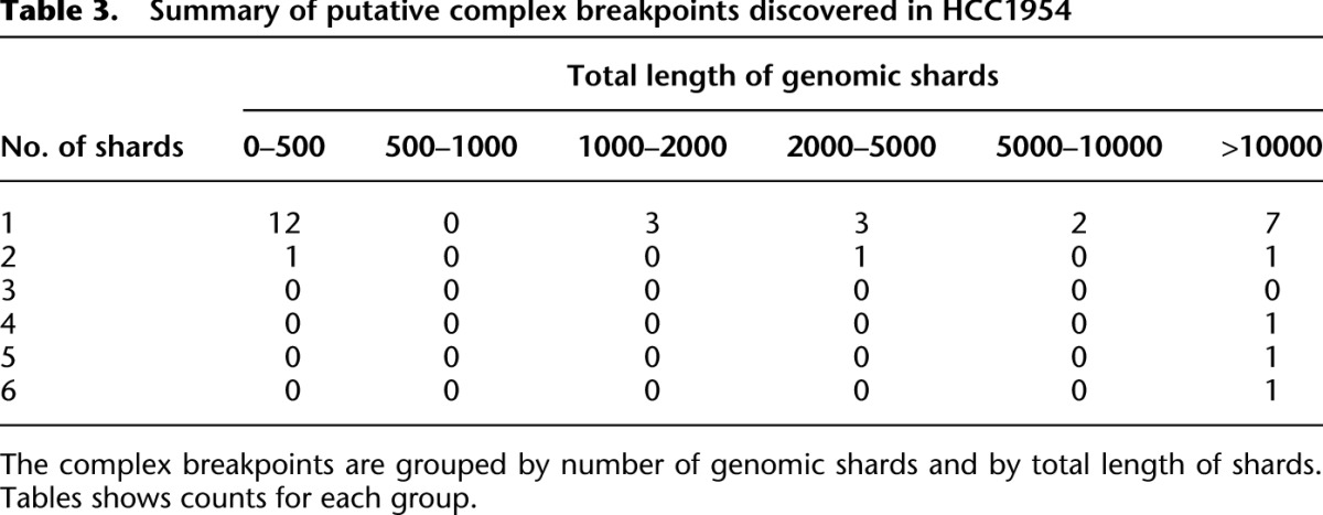
Figure 4.

Complex breakpoints and polyfusions in HCC1954. (A–D) Complex breakpoints produce truncated GSDMC and PVT1 transcripts and _ENDOD1_-WASH2P and _ZDHHC11_-RNF130 fusion transcripts. Validated by LR-PCR. (E) A _PHF20L1_-_FAM49B_-SAMD12 polyfusion produces an in-frame _PHF20L1_-SAMD12 fusion transcript. Validated by LR-PCR. (F–G) Complex breakpoints corroborated by multiple fusion transcripts.
Four of the five validated complex breakpoints (Figs. 4A–D) express intergenic or intronic sequence and are more likely to be truncating mutations than viable fusion genes. The fifth fusion transcript, _PHF20L1_-SAMD12, first discovered by Asmann et al. (2011), is predicted to preserve the reading frames of both PHF20L1 and SAMD12 (Fig. 4E). Among high-confidence fusion transcripts, _PHF20L1_-SAMD12 expression is second only to _STRADB_-NOP58, as suggested by read depth at the breakpoint.
Genomic shards have implications for traditional rearrangement detection techniques. The genomic shards range in size from 220 bp to 4.3 kbp for the five events we validated. A 220-bp genomic shard may be small enough such that some paired end reads span the full complex breakpoint, allowing detection of the breakpoint using conventional methods. However, the 1-kbp and larger genomic shards will be longer than the paired end reads in most WGSS assays, preventing straightforward detection of the breakpoint. Thus a potentially interesting gene fusion such as _PHF20L1_-SAMD12 would be impossible to discover when considering only single breakpoints as evidence for gene fusions, as has been done previously (Bashir et al. 2008). Instead, such methods would falsely nominate _SAMD12_-FAM49B and _PHF20L1_-Intergenic as truncating mutations.
We identified an additional two high-confidence polyfusions by searching for sequences of genomic shards highly connected by fusion transcripts. For each fusion transcript corroborated by alternating path p, we searched for other fusion transcripts corroborated by a subpath of p. We used the resulting sets of (nonconflicting) fusion transcripts to identify polyfusions for which each genomic shard is expressed in at least one nonconflicting fusion transcript. Thus we use fusion transcripts as a scaffold for local genome reconstruction. We believe the highly connected nature of the additional two polyfusions (Figs. 4F,G) provides more confidence in these events.
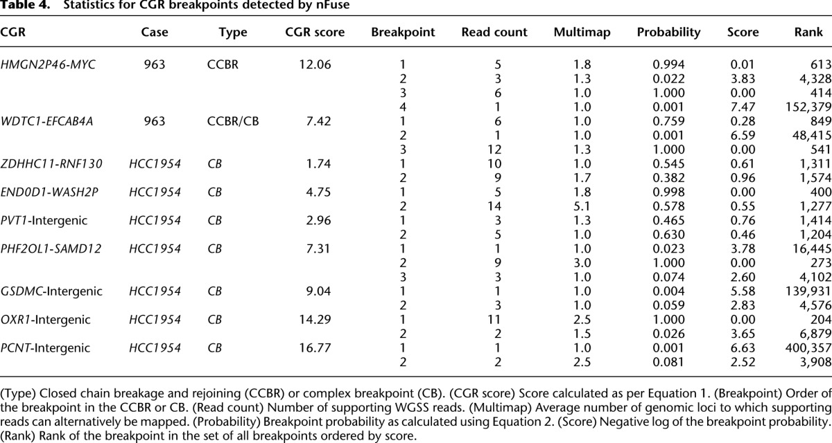
Finally, we used the seven complex breakpoints/polyfusions (five validated and two high-confidence) to evaluate the utility of including suboptimal breakpoint predictions in the breakpoint graph. Statistics for the seven events are detailed in Table 4. The 15 breakpoints for the seven events include breakpoints with low read support, breakpoints supported by multi-map reads, and low probability breakpoints. Three of the breakpoints are supported by only one read. For two of the breakpoints, the entire set of supporting reads also align to other genomic loci and form a coherent cluster at those loci. Thus even multimap resolution methods such as VariationHunter (Hormozdiari et al. 2009) may be unable to identify the correct mappings of these reads. Another two breakpoints are given low probability due to the existence of marginal concordant alignments. Using breakpoints supported by at least two uniquely aligning, high-confidence discordant reads would have resulted in identification of only three of the seven events.
Table 4.
Statistics for CGR breakpoints detected by nFuse
Simulated data set
We used a simulated data set to estimate the sensitivity of the nFuse method. We generated 209 million 80 × 80 WGSS reads and 2.9 million 50 × 50 RNA-seq reads from a simulated genome that included 60 CCBRs and 60 complex breakpoints. WGSS and RNA-seq reads were generated using maq simulate and simulation parameters trained from the HCC1954 data (lanes ERR016395 and ERR022661). The 60 CCBRs and 60 complex breakpoints were generated in three different classes of difficulty, with features of each CGR selected uniformly and at random from a range of values dependent on the class. We analyzed the simulated data set using nFuse with a threshold of 20 for the CGR score.
For the complex breakpoints, we first selected two genes with at least one intron each and then selected an intron from each gene. We created a fusion transcript by splicing the 5′ exons of the first gene to the 3′ exons of the second gene, and we sampled RNA-seq reads from the fusion transcript at a coverage selected from between 20× and 200×. Next we created a complex breakpoint composed of n shards of length {ℓ1..ℓ_n_}, where n and {ℓ1..ℓ_n_} were selected from a range of values dependent on the class difficulty (Table 5). WGSS reads were sampled from the complex breakpoint at a coverage selected from between 5× and 30×. nFuse detected 49 of 60 complex breakpoints in the simulated data set (Table 5).
Table 5.
Complex breakpoints identified in a simulated data set

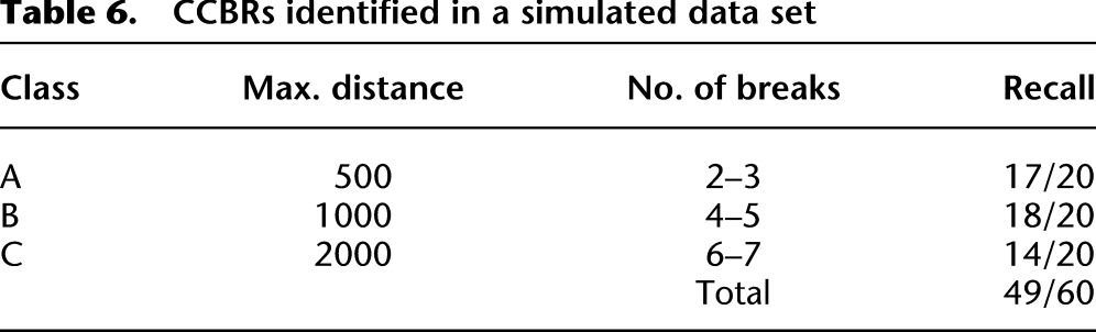
For the CCBRs, we again selected two genes, created a fusion transcript, and generated RNA-seq reads as described above for complex breakpoints. We then simulated a simple breakpoint between the two genes. We also simulated additional n − 1 breakpoints with the structure of a CCBR. Each breakpoint was separated by a distance ℓ_i_ from the subsequent breakpoint in the CCBR. Values for n and {ℓ1..ℓ_n_} were selected from a range of possibilities that depended on the class of difficulty (Table 6). WGSS reads were sampled from the n breakpoints at a coverages selected from between 5× and 30×. nFuse detected 54 of 60 complex breakpoints in the simulated data set (Table 6).
Table 6.
CCBRs identified in a simulated data set
nFuse predicts an additional three CCBRs and four complex breakpoints in the simulated data set. For three of the four false-positive complex breakpoints, the predicted sequence is identical to the sequence of an undiscovered simulated complex breakpoint. However, for each of these three predictions, at least one of the shards is predicted to originate from the wrong location in the genome. Instead, a homologous region is incorrectly predicted as the origin of those shards. The remaining complex breakpoint and three CCBRs also represent undiscovered simulated events with misplaced breakpoints due to homology. Based on the simulation, we estimate the precision of nFuse to be 0.92 for complex breakpoints and 0.95 for CCBRs.
Primary prostate tumor 963
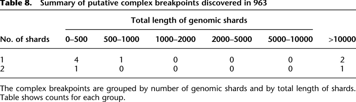
We applied nFuse to the discovery of complex rearrangements in sample 963, a primary prostate tumor sample. We generated WGSS data at 17× physical coverage in addition to 150 million reads of matched RNA-seq (Wu et al. 2012b). The WGSS data produced 762,675 putative breakpoint predictions, and these were used to construct the breakpoint graph for 963. The primary CGR feature of 963 was CCBRs (for summaries of CCBRs and complex breakpoints, respectively, see Tables 7, 8). A four-loci CCBR and three-loci CCBR were prioritized for validation since both affected cancer relevant genes, and each contained a breakpoint supported by only a single read. We validated all breakpoints and fusion transcripts associated with both CCBRs. We also validated a complex breakpoint associated with the three-loci CCBR using LR-PCR. The complex breakpoint and two CCBRs are described in detail below.
Table 7.
Summary of putative CCBRs discovered in 963
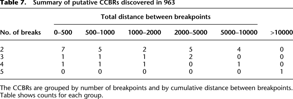
Table 8.
Summary of putative complex breakpoints discovered in 963
As described by Wu et al. (2012b), the 963 tumor is significant because it is difficult to classify in the context of established prostate cancer biology. Although the histology of 963 is consistent with a uniform cell type, the gene expression profile is suggestive of a hybrid luminal/neuroendocrine phenotype. The fusion genes discovered in 963 exhibit a similar hybrid pattern. Some of the fused genes are primarily expressed in luminal cells, and others are primarily expressed in neuroendocrine cells. A growing body of evidence suggests that the binding of transcriptional machinery predisposes DNA to double-stranded breaks (Lin et al. 2009; Nambiar and Raghavan 2011). Thus Wu et al. (2012b) hypothesized that luminal and neuroendocrine expression patterns were present in nascent 963 tumor cells.
Among the catalog of luminal/neuroendocrine fusion genes discovered in 963, two are of particular interest because of their association with a CGR. Most notable of these fusions is highly expressed _HMGN2P46_-MYC, a promoter exchange between the MYC oncogene and luminal cell–specific HMGN2P46, with a breakpoint in MYC similar to that found in Burkitt's lymphoma (Dave et al. 2006). Seemingly unrelated is the _ARHGEF17_-SHANK2 fusion involving neuroendocrine-specific SHANK2, previously reported as fused in melanoma (Berger et al. 2010). We have discovered and validated a CCBR consisting of four breakpoints, one of which produces a _HMGN2P46_-MYC fusion and another that produces a _ARHGEF17_-SHANK2 fusion (Fig. 5A). The discovery of a single genomic event that produces two fusion transcripts, one involving a luminal-specific HMGN2P46 and another involving neuroendocrine specific SHANK2, is evidence that tumorigenesis occurred in a progenitor cell simultaneously expressing both luminal and neuroendocrine specific genes.
Figure 5.

CGRs discovered in primary tumor sample 963. (A) A single CCBR produces four fusion genes: _MYC_-ARHGEF17, _ARHGEF17_-SHANK2, _SHANK2_-HMGN2P46, and _HMGN2P46_-MYC. Only the _ARHGEF17_-SHANK2 and _HMGN2P46_-MYC fusion genes produce fusion transcripts. (B) Example of a CGR that is both a CCBR and a polyfusion involving three loci. The aberrant 1-7-11 chromosome produces three fusion transcripts: _WDTC1_-CD151, _WDTC1_-EFCAB4A, and _WDTC1_-PRKRIP1.
We have also identified a CGR that is represented in the breakpoint graph by a path and a cycle. The path represents a complex breakpoint involving the WDTC1, PRKRIP1, and EFCAB4A genes on chromosomes 1, 7, and 11, respectively. The complex breakpoint was identified as the underlying genomic rearrangement explaining several fusion transcripts. nFuse also identifies a cycle that uses the same two breakpoints as the path, and one additional breakpoint. Given all available information, including fusion transcripts and the three breakpoints, the most parsimonious CGR is a reciprocal translocation between chromosomes 1 and 11, with an insertion of a 800-bp shard of chromosome 7 at one of the breakpoints (Fig. 5B). Without knowledge of the fusion transcripts and given previous interpretation of CCBRs (Berger et al. 2011), the breakpoints may have been interpreted differently. Specifically, the three breakpoints could alternatively represent a transformation that produces three tumor chromosomes: a 1-7 chromosome, a 7-11 chromosome, and an 11-1 chromosome. We are able to exclude this alternate possibility by using the fusion transcripts as a scaffold for local reconstruction of the CGR.
As mentioned in reference to Figure 2B, gain adjacency edges produce CCBRs with ambiguous structures. The gain adjacency edge for _WDTC1_-_PRKRIP1_-EFCAB4A was determined to represent an insertion of a shard of chromosome 7 at a breakpoint between chromosomes 1 and 11, rather than a region of chromosome 7 duplicated in two tumor chromosomes. Thus we sought to rule out the possibility that all gain adjacency edges represent insertions. The MYC CCBR includes two gain adjacency edges. If either of these gain edges represented insertions, it would be impossible for the MYC CCBR alone to explain the _ARHGEF17_-SHANK2 and _HMGN2P46_-MYC fusion transcripts; additional breakpoints and further complexity would be required. Thus the most parsimonious explanation is that the gain adjacency edges of the MYC CCBR represent regions of chromosome 11 that are duplicated in the final tumor chromosomes.
Discussion
We have applied nFuse to the discovery of fusion transcripts and underlying CGRs in breast cancer cell line HCC1954 and a primary prostate tumor sample 963. The landscape of CGR events differed between HCC1954 and 963, with complex breakpoints and polyfusions arising as the predominant CGR feature of HCC1954, and CCBRs arising as the predominant feature of 963. In HCC1954, nFuse predicted seven high-confidence complex breakpoints/polyfusions. One of these fusions is _PHF20L1_-SAMD12, a highly expressed in-frame fusion missed by Stephens et al. (2009) likely because of the complexity of the breakpoint. In fact, our results strongly suggest that analysis of single breakpoints in isolation is inadequate as a method for identifying fusion genes. The large size of fragments that are interposed at the breakpoints of some fusion genes will prevent the discovery of those fusions. nFuse is also capable of identifying the single breakpoints underlying fusion transcripts caused by more simple rearrangements. nFuse successfully recovers all four fusion transcripts identified by ShowShoes-FTD, predicting a simple rearrangement for three and a CGR for the forth.
In 963, nFuse identified a CGR with potential biological implications. Based on existing evidence that transcribed genes are prone to double-stranded breaks and building on the suggestion by Berger et al. (2011) that CCBRs occur for sets of genes recruited to the same transcriptional factory, we propose that CCBRs may be used to infer the gene coexpression history of a tumor. In 963, the discovery of the MYC CCBR suggests that luminal-specific HMGN2P46 and neuroendocrine-specific SHANK2 were coexpressed in a single nascent tumor cell during the formation of the CCBR. Thus the CCBR provides further evidence of the dual luminal/neuroendocrine history of the 963 tumor and suggests the unusual luminal/neuroendocrine expression pattern of the tumor predates the formation of the MYC rearrangement.
We have used examples in both HCC1954 and 963 to highlight the potential utility of performing an integrated analysis of matched WGSS and RNA-seq data sets. The RNA-seq data yield information about long-range connectivity between genomic regions, acting as a set of very long genomic reads. As such, the RNA-seq data can be useful as a scaffold for reconstructing tumor chromosomes. In some cases the RNA-seq data can also be used to resolve genomic architectural ambiguities, as for the two CCBRs discussed for 963. Finally, RNA-seq can be used to identify potentially interesting events such as fusion transcripts that serve as a starting point for targeted analysis.
Many fusion genes, including those with complex origins such as _PHF20L1_-SAMD12, can be detected using conventional analysis of RNA-seq data. Nevertheless, many interesting questions cannot be answered with a fusion transcript prediction alone. For instance, it is impossible to measure the clonal abundance of a gene fusion at the transcriptomic level alone, since transcript abundance is heavily influenced by expression. Given multiple tumor samples from the same patient, knowledge of breakpoints will allow us to ask which samples harbor the fusion, whereas knowledge of the fusion transcript only allows us to understand the expression levels in each sample. Furthermore, an understanding of the clonal abundances of rearrangements will help determine the evolutionary history of the tumor. The evolutionary history will then help determine the founder status of each rearrangement, and which rearrangements are drivers of tumorigenesis (Shah et al. 2012).
Finally, it has been assumed throughout this work that the breakpoints of CGRs occur simultaneously during a single event. A complex breakpoint with one genomic shard could also be formed by a two independent breakage-rejoining events that occur at the same loci at different times during the tumors development. Similarly, a CCBR could be formed by breakage and rejoining events occurring in succession at the same loci. Both of these scenarios require the formation of intermediate breakpoints. In the evolutionary history of the tumor, some cells would likely have evolved from cells in the intermediate state without having gained all breakpoints in the CGR. Thus we expect the intermediate breakpoints to be present in some proportion of tumor cells, though that proportion may be very small. To date we have not identified any intermediate breakpoints in the sequencing data. Future work will involve testing for intermediate breakpoints, and negative results will provide further evidence of the simultaneity of CGRs.
Data access
The nFuse source code and manual can be downloaded at http://nfuse.googlecode.com.
Acknowledgments
This work was supported in part by the Natural Sciences and Engineering Research Council of Canada (NSERC), Bioinformatics for Combating Infectious Diseases (BCID) grants to S.C.S., NSERC Alexander Graham Bell Canada Graduate Scholarships (CGS-D) to A.M., and the CIHR/MSFHR Strategic Training Program in Bioinformatics.
Footnotes
[Supplemental material is available for this article.]
References
- Asmann YW, Hossain A, Necela BM, Middha S, Kalari KR, Sun Z, Chai HS, Williamson DW, Radisky D, Schroth GP, et al. 2011. A novel bioinformatics pipeline for identification and characterization of fusion transcripts in breast cancer and normal cell lines. Nucleic Acids Res 39: e100 doi: 10.1093/nar/gkr362 [DOI] [PMC free article] [PubMed] [Google Scholar]
- Bashir A, Volik S, Collins C, Bafna V, Raphael BJ 2008. Evaluation of paired-end sequencing strategies for detection of genome rearrangements in cancer. PLoS Comput Biol 4: e1000051 doi: 10.1371/journal.pcbi.1000051 [DOI] [PMC free article] [PubMed] [Google Scholar]
- Berger MF, Levin JZ, Vijayendran K, Sivachenko A, Adiconis X, Maguire J, Johnson LA, Robinson J, Verhaak RG, Sougnez C, et al. 2010. Integrative analysis of the melanoma transcriptome. Genome Res 20: 413–427 [DOI] [PMC free article] [PubMed] [Google Scholar]
- Berger MF, Lawrence MS, Demichelis F, Drier Y, Cibulskis K, Sivachenko AY, Sboner A, Esgueva R, Pflueger D, Sougnez C, et al. 2011. The genomic complexity of primary human prostate cancer. Nature 470: 214–220 [DOI] [PMC free article] [PubMed] [Google Scholar]
- Bignell GR, Santarius T, Pole JC, Butler AP, Perry J, Pleasance E, Greenman C, Menzies A, Taylor S, Edkins S, et al. 2007. Architectures of somatic genomic rearrangement in human cancer amplicons at sequence-level resolution. Genome Res 17: 1296–1303 [DOI] [PMC free article] [PubMed] [Google Scholar]
- Chen K, Wallis JW, McLellan MD, Larson DE, Kalicki JM, Pohl CS, McGrath SD, Wendl MC, Zhang Q, Locke DP, et al. 2009. BreakDancer: An algorithm for high-resolution mapping of genomic structural variation. Nat Methods 6: 677–681 [DOI] [PMC free article] [PubMed] [Google Scholar]
- Dave SS, Fu K, Wright GW, Lam LT, Kluin P, Boerma EJ, Greiner TC, Weisenburger DD, Rosenwald A, Ott G, et al. 2006. Molecular diagnosis of Burkitt's lymphoma. N Engl J Med 354: 2431–2442 [DOI] [PubMed] [Google Scholar]
- Galante P, Parmigiani R, Zhao Q, Caballero O, de Souza J, Navarro F, Gerber A, Nicolás M, Salim A, Silva A, et al. 2011. Distinct patterns of somatic alterations in a lymphoblastoid and a tumor genome derived from the same individual. Nucleic Acids Res 39: 6056–6068 [DOI] [PMC free article] [PubMed] [Google Scholar]
- Greenman CD, Pleasance ED, Newman S, Yang F, Fu B, Nik-Zainal S, Jones D, Lau KW, Carter N, Edwards PA, et al. 2011. Estimation of rearrangement phylogeny for cancer genomes. Genome Res 22: 346–361 [DOI] [PMC free article] [PubMed] [Google Scholar]
- Hormozdiari F, Alkan C, Eichler EE, Sahinalp SC 2009. Combinatorial algorithms for structural variation detection in high-throughput sequenced genomes. Genome Res 19: 1270–1278 [DOI] [PMC free article] [PubMed] [Google Scholar]
- Hormozdiari F, Hajirasouliha I, McPherson A, Eichler EE, Sahinalp SC 2011. Simultaneous structural variation discovery among multiple paired-end sequenced genomes. Genome Res 21: 2203–2212 [DOI] [PMC free article] [PubMed] [Google Scholar]
- Langmead B, Salzberg S 2012. Fast gapped-read alignment with bowtie 2. Nat Methods 9: 357–359 [DOI] [PMC free article] [PubMed] [Google Scholar]
- Lin C, Yang L, Tanasa B, Hutt K, Ju B, Ohgi K, Zhang J, Rose D, Fu X, Glass C, et al. 2009. Nuclear receptor-induced chromosomal proximity and dna breaks underlie specific translocations in cancer. Cell 139: 1069–1083 [DOI] [PMC free article] [PubMed] [Google Scholar]
- McPherson A, Hormozdiari F, Zayed A, Giuliany R, Ha G, Sun M, Griffith M, Heravi Moussavi A, Senz J, Melnyk N, et al. 2011a. deFuse: An algorithm for gene fusion discovery in tumor RNA-Seq data. PLoS Comput Biol 7: e1001138 doi: 10.1371/journal.pcbi.1001138 [DOI] [PMC free article] [PubMed] [Google Scholar]
- McPherson A, Wu C, Hajirasouliha I, Hormozdiari F, Hach F, Lapuk A, Volik S, Shah S, Collins C, Sahinalp C, et al. 2011b. Comrad: Detection of expressed rearrangements by integrated analysis of RNA-Seq and low coverage genome sequence data. Bioinformatics 27: 1481–1488 [DOI] [PubMed] [Google Scholar]
- Mitelman F, Johansson B, Mertens F 2007. The impact of translocations and gene fusions on cancer causation. Nat Rev Cancer 7: 233–245 [DOI] [PubMed] [Google Scholar]
- Nambiar M, Raghavan S 2011. How does DNA break during chromosomal translocations? Nucleic Acids Res 39: 5813–5825 [DOI] [PMC free article] [PubMed] [Google Scholar]
- Ozery-Flato M, Shamir R 2009. Sorting cancer karyotypes by elementary operations. J Comput Biol 16: 1445–1460 [DOI] [PubMed] [Google Scholar]
- Pevzner P. 2000 Computational molecular biology: An algorithmic approach (Computational Molecular Biology). MIT Press, Cambridge, MA. [Google Scholar]
- Raphael BJ, Pevzner PA 2004. Reconstructing tumor amplisomes. Bioinformatics 20: 265–273 [DOI] [PubMed] [Google Scholar]
- Raphael BJ, Volik S, Collins C, Pevzner PA 2003. Reconstructing tumor genome architectures. Bioinformatics 19: 162–171 [DOI] [PubMed] [Google Scholar]
- Shah S, Roth A, Goya R, Oloumi A, Ha G, Zhao Y, Turashvili G, Ding J, Tse K, Haffari G, et al. 2012. The clonal and mutational evolution spectrum of primary triple-negative breast cancers. Nature 486: 395–399 [DOI] [PMC free article] [PubMed] [Google Scholar]
- Stephens PJ, McBride DJ, Lin ML, Varela I, Pleasance ED, Simpson JT, Stebbings LA, Leroy C, Edkins S, Mudie LJ, et al. 2009. Complex landscapes of somatic rearrangement in human breast cancer genomes. Nature 462: 1005–1010 [DOI] [PMC free article] [PubMed] [Google Scholar]
- Stephens P, Greenman C, Fu B, Yang F, Bignell G, Mudie L, Pleasance E, Lau K, Beare D, Stebbings L, et al. 2011. Massive genomic rearrangement acquired in a single catastrophic event during cancer development. Cell 144: 27–40 [DOI] [PMC free article] [PubMed] [Google Scholar]
- Tuzun E, Sharp AJ, Bailey JA, Kaul R, Morrison VA, Pertz LM, Haugen E, Hayden H, Albertson D, Pinkel D, et al. 2005. Fine-scale structural variation of the human genome. Nat Genet 37: 727–732 [DOI] [PubMed] [Google Scholar]
- Volik S, Zhao S, Chin K, Brebner JH, Herndon DR, Tao Q, Kowbel D, Huang G, Lapuk A, Kuo WL, et al. 2003. End-sequence profiling: Sequence-based analysis of aberrant genomes. Proc Natl Acad Sci 100: 7696–7701 [DOI] [PMC free article] [PubMed] [Google Scholar]
- Wang J, Mullighan CG, Easton J, Roberts S, Heatley SL, Ma J, Rusch MC, Chen K, Harris CC, Ding L, et al. 2011. CREST maps somatic structural variation in cancer genomes with base-pair resolution. Nat Methods 8: 652–654 [DOI] [PMC free article] [PubMed] [Google Scholar]
- Wu C, Wyatt AW, McPherson A, Lin D, McConeghy BJ, Mo F, Shukin R, Lapuk AV, Jones SJM, Zhao Y, et al. 2012a. Poly-gene fusion transcripts and chromothripsis in prostate cancer. Genes Chromosomes Cancer. doi: 10.1002/gcc.21999 [DOI] [PubMed] [Google Scholar]
- Wu C, Wyatt AW, Lapuk AV, McPherson A, McConeghy BJ, Bell RH, Anderson S, Haegert A, Brahmbhatt S, Shukin R, et al. 2012b. Integrated genome and transcriptome sequencing identifies a novel form of hybrid and aggressive prostate cancer. J Pathol 227: 53–61 [DOI] [PMC free article] [PubMed] [Google Scholar]
- Zhao Q, Caballero OL, Levy S, Stevenson BJ, Iseli C, de Souza SJ, Galante PA, Busam D, Leversha MA, Chadalavada K, et al. 2009. Transcriptome-guided characterization of genomic rearrangements in a breast cancer cell line. Proc Natl Acad Sci 106: 1886–1891 [DOI] [PMC free article] [PubMed] [Google Scholar]
- Zhao Q, Kirkness E, Caballero O, Galante P, Parmigiani R, Edshall L, Kuan S, Ye Z, Levy S, Vasconcelos A, et al. 2010. Systematic detection of putative tumor suppressor genes through the combined use of exome and transcriptome sequencing. Genome Biol 11: R114 doi: 10.1186/gb-2010-11-11-r114 [DOI] [PMC free article] [PubMed] [Google Scholar]