Force Spectroscopy with Dual-Trap Optical Tweezers: Molecular Stiffness Measurements and Coupled Fluctuations Analysis (original) (raw)
Abstract
Dual-trap optical tweezers are often used in high-resolution measurements in single-molecule biophysics. Such measurements can be hindered by the presence of extraneous noise sources, the most prominent of which is the coupling of fluctuations along different spatial directions, which may affect any optical tweezers setup. In this article, we analyze, both from the theoretical and the experimental points of view, the most common source for these couplings in dual-trap optical-tweezers setups: the misalignment of traps and tether. We give criteria to distinguish different kinds of misalignment, to estimate their quantitative relevance and to include them in the data analysis. The experimental data is obtained in a, to our knowledge, novel dual-trap optical-tweezers setup that directly measures forces. In the case in which misalignment is negligible, we provide a method to measure the stiffness of traps and tether based on variance analysis. This method can be seen as a calibration technique valid beyond the linear trap region. Our analysis is then employed to measure the persistence length of dsDNA tethers of three different lengths spanning two orders of magnitude. The effective persistence length of such tethers is shown to decrease with the contour length, in accordance with previous studies.
Introduction
Optical tweezers (OT) have been often employed to measure the elastic properties of polymers tethered between dielectric beads. A direct measurement of the tether stiffness is possible through fluctuation analysis (1). This kind of measurement is appealing from the experimental point of view because they require the measurement of a single quantity, either force or extension, so that they do not need a prior determination of the trap stiffness. One major source of error in these measurements is the coupling of fluctuations along different spatial directions, mainly in and out of the focal plane. This is a nontrivial effect that is expected to affect (although to different extents) any OT setup. The relevance of such effect is not limited to fluctuation measurements: it can also affect the correct measurement of force-extension curves, especially for short tethers. A clear understanding of the physical basis of such couplings is useful to determine under which conditions they lead to systematic errors in the measurements.
In this article, we study fluctuation coupling in double-trap optical-tweezers (DTOT) setups commonly used in high-resolution force spectroscopy. The most important coupling sources are misalignment effects affecting both traps and tether. Through theoretical modeling, we establish a criterion to identify the kind of misalignment that causes the coupling and give explicit formulas to quantify its effect based on the parameters characterizing the experimental setup. These considerations are also relevant for single-trap optical tweezers (STOT). Moreover, we show that, if coupling effects are negligible, the analysis of the variance of the measured signals, either force or position, may be used to simultaneously measure the tether and trap stiffnesses, including possible asymmetries between the two traps.
This kind of measurement can be used as a calibration technique, suitable for any DTOT, which works beyond the linear region of the traps. When instead couplings are nonnegligible, we show how to include them in the data analysis. To illustrate this methodology we carried out measurements in a, to our knowledge, novel DTOT setup that uses counterpropagating beams and measures forces directly using linear momentum conservation. This system is especially well suited for stiffness measurements as the force measurement calibration is independent of the shape and size of the trapped object. This is not true when using other techniques, e.g., back-focal plane interferometry, which require a specific calibration of the position measurement for each bead. We performed direct measurements of the stiffness of dsDNA tethers whose contour length spans two decades.
Materials and Methods
Optical tweezers setup
The DTOT setup is shown in Fig. 1 and is very similar to the one designed by Smith et al. (2) and described in Huguet et al. (3), which operates with a single trap and a pipette. Force measurement is based on the conservation of linear momentum (2), making force calibration very robust. Calibration factors are determined by the optical setup and the detector response but they are independent of other details of the experimental setup, such as the index of refraction of the trapped object, its size or shape, the refractive index of the buffer medium, and laser power. Unless the optics or the detector are changed, there is no need for continued calibration (2). Fluctuation measurements were performed using an acquisition board (Agilent Technologies, Santa Clara, CA) with a 50 kHz bandwidth, which is higher than corner frequencies of the measured signals. In a typical experiment, fluctuations were measured for 10 s, by increasing the force in 2-pN steps between subsequent measurements.
Figure 1.
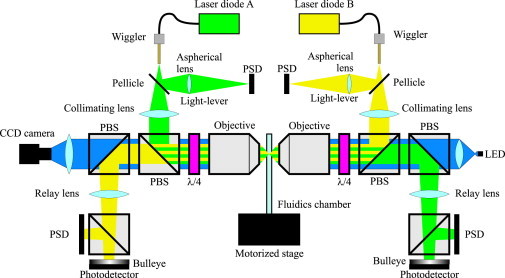
Experimental setup. The scheme of the optical setup, with the optical paths of the lasers and the LED. Fiber-coupled diode lasers are focused inside a fluidics chamber to form optical traps using underfilling beams in high NA objectives. All the light leaving from the trap is collected by a second objective, and sent to a position-sensitive detector that integrates the light momentum flux, measuring changes in light momentum (2). The laser beams share part of their optical paths and are separated by polarization. Part of the laser light (≃ 5%) is deviated by a pellicle before focusing and used to monitor the trap position (light lever). Each trap is moved by pushing the tip of the optical fiber by piezos coupled to a brass tube (wigglers).
Molecular synthesis
For our experiments, we used dsDNA tethers of four different lengths. The 24 kb tether was obtained by digesting the phage-λ plasmid with the _XbA_I restriction enzyme. The tether was then ligated to a biotin-labeled oligo on one side and with a dig-labeled oligo on the other side. The 3 kb tether was obtained by PCR amplification of a section of the phage-λ plasmid using biotin-modified primers. The amplified segment was then restricted with _Xba_I and ligated to a dig-modified oligo. The 1.2 kb and 58 b tethers were synthesized according to the protocol described in Forns et al. (4). Experiments were performed in a microfluidic chamber formed by two coverslips interspaced with parafilm. Anti-dig coated beads were first incubated with the molecule of interest and then introduced one at a time in the microfluidics chamber through a dispenser tube. Once the anti-dig coated bead was trapped, a streptavidin-coated bead was introduced through a second dispenser tube and trapped in the second trap. The connection was then formed directly inside the microfluidics chamber. All experiments on DNA tethers were performed in phosphate-buffered saline solution at pH 7.4, NaCl 1 M, at 25°C. This buffer solution was found to greatly reduce the nonspecific adsorption of DNA on silica. We dissolved 1 mg/_μ_L bovine serum albumin in the buffer to reduce nonspecific silica-silica interactions.
Results
Coupled fluctuations in a plane
To introduce the main subject of this article, it is useful to consider a pedagogical example that shows how a small coupling between two fluctuating degrees of freedom can have a large effect on their variances. Let us consider a particle moving on a plane while constrained by two harmonic springs (Fig. 2 A). The position of the particle is given by a vector p = (y,z) and the springs are oriented along the coordinate axes (yˆ,zˆ) (Fig. 2 A). The stiffness matrix k¯ is given by
| k¯=(ky00kz)=ky(100α),α=kzky, | (1) |
|---|
where k y,k z are the stiffnesses along y,z, respectively. The equilibrium Boltzmann distribution for p can be written in compact form as
| ρ(p)=1Zexp(−p·k¯p2kBT), | (2) |
|---|
| Z=∫dzdyexp(−p·k¯p2kBT), | (3) |
|---|
where _k_B is the Boltzmann constant, T is the absolute temperature, and Z is the partition function. The variance of p is thus
| 〈p2〉=kBTk¯−1≃kBTky(1001α). | (4) |
|---|
In the case k y ≫ k z (α ≪ 1), the variance of spatial fluctuations along z is much bigger than the variance along y and the level curves of the probability distribution in Eq. 2 are highly eccentric ellipses (Fig. 2 C, red solid curves).
Figure 2.
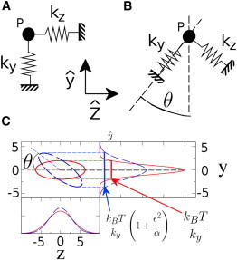
Coupled fluctuations in a plane. (A) A particle (P) is constrained by two springs that are oriented along the y,z coordinate axes (shown by the two arrows). The values k y,k z denote the spring stiffnesses along y,z. (B) A particle (P) constrained by two springs that are misaligned by an angle θ with respect to the coordinate axes. (C) Level curves and marginal distributions for the joint equilibrium probability distribution of the particle position in the two systems shown in panels A (solid curves) and B (dashed curves). If the two springs have very different stiffnesses, the level curves form highly eccentric ellipses. In this situation a rotation by a small angle θ in the joint distribution can lead to a large change in the marginal distribution for y. The large difference in stiffness acts as a lever arm amplifying the strength of the coupling.
If the springs are misaligned by an angle θ with respect to the reference frame (Fig. 2 B), the stiffness tensor changes as
| k′¯=R¯(θ)k¯R¯T(θ)=(kycos2θ+kzsin2θ(ky−kz)cosθsinθ(ky−kz)cosθsinθkzcos2θ+kysin2θ), | (5) |
|---|
where k′¯ is the new stiffness and R¯(θ) is a rotation of angle θ. In this situation, because k y ≠ k z, the off-diagonal terms in Eq. 5 couple the motion of the particle along y and z. We define ε = sin_θ_ as the coupling parameter. To lowest order in ε, we get
| 〈p2〉=kBTk¯′−1≃kBTky(1+(1α−1)ϵ2ϵ(1−1α)ϵ(1−1α)1α(1−ϵ2)+ϵ2). | (6) |
|---|
For a small coupling ε, the variance of y is increased to
| 〈y2〉=kBTky(1+(1α−1)ϵ2)≃kBTky(1+ϵ2α),(α≪1). | (7) |
|---|
This shows that the effect of a small coupling ε (small misalignment of the springs) on the variance of y can be large if ϵ2/α∼1. In other words, the small _α_-value acts as a lever arm, amplifying the effect of a small rotation (Fig. 2 C). Only when
can the coupling of fluctuations be ignored. So far, we gave the general picture of the effect of a coupling between two fluctuating degrees of freedom. In the next section, we will show how this simple model can be extended to study fluctuations in a DTOT. Generally speaking, when a molecule is pulled at high forces the rigidity of the tether is much higher along the pulling direction (y) than in the perpendicular direction (z) and Eq. 8 can be violated even if ε is very small (≃ 0.1). At low forces and for long tethers, Eq. 8 is instead fulfilled and the coupling can be ignored. A quantitative treatment of these effects and the corresponding data analysis are described next.
Coupled fluctuations in a DTOT setup
Correlation functions of fluctuation measurements in a DTOT do often show a double-exponential nature. This is usually interpreted in terms of a coupling of the fluctuations in the optical plane and along the optical axis (5,6). Couplings affect the variance of the measured force (or position) signal and the spurious contribution must be removed from the measurements. Yet, coupling effects reflect some defect in the design of the experimental setup and their study can provide valuable diagnostic tools for the fine tuning of a DTOT setup, crucial for high-resolution measurements.
Most prominent coupling sources are misalignment effects, due to at least two causes:
A first cause is tether misalignment, i.e., a configuration in which the centers of the traps lie in different planes (Fig. 3 C).
Figure 3.
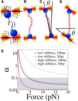
Misaligned experimental configurations. (A) The coordinate system used throughout the text. The direction of light propagation (black horizontal arrows) defines the optical (zˆ) axis. The stretching direction, perpendicular to zˆ, defines the yˆ axis. The positions of the beads ((_y_1,_z_1) and (_y_2,_z_2)) are measured with respect to the equilibrium positions and _r_0 denotes the mean separation between the centers of the beads. (B) In the aligned configuration, the tether is perfectly oriented along the yˆ axis. (C) Misaligned tether, the two traps are focused at different positions along the optical axis and the tether forms an angle θ with the yˆ axis. (D) In misaligned traps, the principal axes of the traps form an angle θ with the _y_-z reference frame. (E) The value of α, Eq. 28, as a function of the mean force, for different tethers (3 kbp and 24 kbp dsDNA) and trap stiffnesses. (Continuous lines, i.e., low trap stiffness) Setup similar to that used for the measurements discussed in this article, with k y ≃ 0.02 pN/nm, k z ≃ 0.01 pN/nm. (Dotted line, i.e., high trap stiffness) Setup 10-times stiffer (such as that described in Gebhardt et al. (7) and Comstock et al. (8)). (Shaded area) Values of α for which a coupling ε ≃ 0.1 causes a 10% error (_ε_2/α ≃ 0.1).
A second case is trap misalignment, when the principal axes of the traps are tilted with respect to the direction along which the tether is stretched (Fig. 3 D).
Remarkably, these two scenarios lead to different coupling structures making possible the identification of misalignment effects. To discuss coupling effects, it is necessary to consider a four-dimensional configuration space, describing the position of the beads both along the optical axis and the pulling direction. The laser beams (_black arrow_s in Fig. 3 A) define the optical axis, which we identify with the zˆ direction in our reference frame. In the optical plane (perpendicular to the optical axis), we shall use the coordinate yˆ to denote the direction along which the tether is oriented. The coordinate xˆ, perpendicular to both yˆ and zˆ, will play no role in our analysis. The effect of both traps and tether on the dynamics of the beads can be modeled by a potential energy function, which depends on the positions of the beads in the y_–_z plane. When considering equilibrium fluctuations at constant trap-to-trap distance, a linear approximation around the equilibrium positions can be used,
| U(y1,y2,z1,z2)=12pTK′¯p, | (9) |
|---|
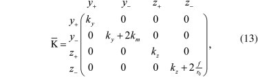
with p = (_y_1, _y_2, _z_1, _z_2), and K′¯ the stiffness tensor (tensors are primed when they are represented in the y_–_z coordinate system). In the ideal case (Fig. 3 B), the stiffness tensor, which is now 4 × 4, readsThe stiffness tensor is two-block diagonal, with the first block describing the effect of traps and tether along the y axis, and the second block describing the effect of traps and tether in the zˆ direction, sharing the same structure. Here k y is the stiffness of the trap in the yˆ direction (the two traps are assumed identical for simplicity), k z is the trap stiffness in the zˆ direction, k m is the stiffness of the tether connecting the two beads, f is the mean force, and _r_0 is the mean distance between the centers of the beads. In this case, the stiffness tensor can be diagonalized, switching to the coordinate system defined by
| y+=y1+y22,y−=y1−y22, | (11) |
|---|
| z+=z1+z22,z−=z1−z22, | (12) |
|---|
where y+,z+ represent the center-of-mass position and _y_−,_z_− represent the differential coordinate. In this second coordinate system, the stiffness tensor readswhich shows that the four different fluctuation modes are uncoupled (we dropped the prime because we switched to a different reference frame). The tensor K¯ can be written as the sum of two contributions,
with
| K¯T=(ky0000ky0000kz0000kz), | (15) |
|---|
which accounts for the trap contribution to the stiffness, and
| K¯m=(00000km000000000fr0), | (16) |
|---|
which accounts for the tether contribution to the stiffness.
Tether misalignment effects
In the presence of tether misalignment, i.e., if the two traps are focused at different depths along the optical axis (Fig. 3 C), the tether forms an angle θ with respect to the y axis. This can be incorporated in the stiffness tensor through a rotation of K¯m, Eq. 16, of the same angle:
| K¯m(ϵ)=(00000u(ϵ)0ϵw(ϵ)00000ϵw(ϵ)0v(ϵ)), | (17) |
|---|
with
and ε = sin(θ).
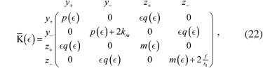
The total stiffness tensor is nowwhich must be compared to Eq. 13. Looking at the nondiagonal terms of this tensor, it is evident that the coupling will only affect the two differential modes, _y_−,_z_−, leaving the motion of the center of mass, y+,z+, unchanged.
Trap misalignment effect
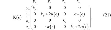
In the second configuration, the trap stiffness tensor is rotated (Fig. 3 D), and the stiffness tensor becomes
with
and ε = sin(θ). In contrast to the previous case, the nondiagonal terms show that the coupling will affect both the differential and center-of-mass coordinates. This important difference provides a simple tool to distinguish between tether and trap misalignments.
On the relevance of coupling effects
In the case of tether misalignment, the off-diagonal terms in Eq. 21 couple the fluctuations along the _y_− and _z_− directions. A reduced description addressing these two coordinates is possible using a subtensor of K¯(ϵ) (see Eq. 21):

The variance of _y_− is given by
| 〈y−2〉=kBT(K′¯−(ϵ)−1)y−y−, | (27) |
|---|
which, to leading order in ε, is
with
| α=(ky+2km)(kz+2f/r0)(2km+kz)(2km−2f/r0). | (29) |
|---|
The value of α can be computed if the stiffnesses are known. In Fig. 3 E, we show the behavior of α as a function of the force for two different dsDNA tethers (3 kbp and 24 kbp) and for two different trap stiffnesses. The continuous curves show the value of α computed in a low stiffness setup (k y = 0.02 pN/nm, k z = 0.001 pN/nm, the condition in which our DTOT operates) whereas the dotted lines show the value of α for high trap stiffness (k y = 0.2 pN/nm, k z ≃ 0.01 pN/nm, as reported for the DTOT in Gebhardt et al. (7) and Comstock et al. (8)). Even in the case of high trap stiffness, the attained value of α is small (≃10−1) at high forces for the shorter tether. In Fig. 3 E, the shaded area shows the values of α for which a misalignment ε ≃ 0.1 causes a 10% error in the measurements of _y_− fluctuations Eq. 28. In our DTOT setup, such coupling in negligible when using long molecules (8 _μ_m) at low and moderate forces (up to ≃10 pN).
In the case of trap misalignment, both the variances of _y_− and y+ are affected and similar formulas hold:
| 〈y−2〉〈y−2〉ϵ=0=1+ϵ2γ〈y+2〉〈y+2〉ϵ=0=1+ϵ2δ, | (30) |
|---|
| γ=(ky+2km)(kz+2f/r0)(ky−kz)(ky+2f/r0), | (31) |
|---|
Equations 28, 31, and 32 estimate the error due to misalignment as a function of the stiffnesses contributing to the experimental setup (Fig. 3 E). As such, they are useful to understand in which force regimes misalignment is going to be important.
Neglecting coupling effects: variance analysis
In experimental setups where force is directly measured, the trap stiffness is used to measure the extension of the fiber. Conversely, when the bead displacement is measured (e.g., by video microscopy or by back-focal-plane interferometry (9)), the stiffness is used to measure force. In both cases, the trap stiffness depends on the details of the experimental setup, i.e., laser power, bead size, and shape or buffer medium (via its refraction index). Optical traps are assumed to be linear close to the trap center, so that a stiffness measurement at zero force can be used to characterize the trap shape in this region. This kind of calibration has been shown to achieve 1% accuracy (10). Nevertheless, when one needs to do measurements at high forces, nonlinear effects may become relevant, especially at low trap power and the full force field of the trap should be measured (11).
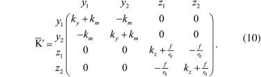
When the coupling is negligible, motions along the yˆ and zˆ directions are uncoupled and the stiffnesses of traps and tethers can be obtained from a straightforward analysis of the experimental force (or position) variances. We will model traps and tether by the dumbbell shown in Fig. 4. It consists of three serially connected harmonic springs. In this setting we allow for a different stiffness in the two traps: _k_1, _k_2 (Fig. 4 A). Together with the tether stiffness k m we get the stiffness tensor,
| K′¯=(k1+km−km−kmk2+km), | (33) |
|---|
which is just the first block of Eq. 10, and the potential energy of the system is written as
| U(y1,y2)=12(y1,y2)·K′¯(y1,y2), | (34) |
|---|
where (_y_1,_y_2) have the same meaning as in the previous sections. The equilibrium distribution for (_y_1,_y_2) is related to K′¯ by
| P(y1,y2)=1Zexp(−U(y1,y2)kBT). | (35) |
|---|
The variances and covariance of (_y_1,_y_2) are linked to the inverse of the stiffness tensor. In terms of the experimentally measured variances and covariances,
| k1=κ〈y22〉−〈y1y2〉kBT, | (36) |
|---|
| k2=κ〈y12〉−〈y1y2〉kBT, | (37) |
|---|
with
κ−1=〈y12〉〈y22〉−〈y1y2〉2(kBT)2.
Figure 4.
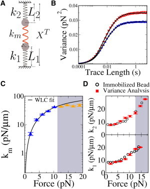
Trap and molecular stiffness measurements. (A) A linear dumbbell model, where three elastic elements with different stiffnesses are arranged in series: Trap 1 (_k_1), Trap 2 (_k_2), and the tether (k m). (B) Measured force variance as a function of trace length. The two data sets refer to the variance in each trap, measured on a 24-kbp tether and pulled at 10 pN. Force fluctuations in each trap are the superposition of two different linear modes. (Solid curves) Fits to the expected behavior in the case of a superposition of two modes (see the Supporting Material). The good agreement between theory and experiment shows that the effect of low-frequency noise is not relevant on our experimental timescales (<1%). (C) Molecular stiffness (k m) measured and averaged over different molecules. (Continuous line) Fit to the extensible WLC model Eq. 44, giving a persistence length P = 52 ± 4 nm and a stretch modulus S = 1000 ± 200 pN, consistent with what it is reported in Smith et al. (19). (Shaded area) Region where misalignment is expected to be relevant. The fair points are not included in the fit and show the effect of misalignment. (D) Comparison of the stiffness values of the two traps, _k_1 and _k_2, measured through Eqs. 39–41 (solid symbols) with those measured by immobilizing the bead on the micropipette (open symbols); see Materials and Methods. Measurements agree within experimental errors. Note that stiffness is measured correctly even when misalignment is relevant (shaded region). This happens because the measurement of trap stiffness is mostly based on the center-of-mass coordinate, which is not affected in the case of tether misalignment.
In experimental setups that directly measure forces, different formulas apply: the experimental values (_σ_211, _σ_222, σ_212, σ_2_ij = 〈_f i f j_〉−〈_f i_〉〈_f _j_〉, i = 1,2) and the model parameters (_k_1, _k_2, k m) are related by
| km=1kBTσ122(σ112+σ122)(σ222+σ122)σ112σ222−σ124. | (41) |
|---|
The method we have introduced in this section is similar to the one used by Meiners and Quake (1), the difference being that here we use equal-time force covariance whereas Meiners and Quake (1) uses time-dependent correlation functions. Both methods can be affected by the presence of extraneous noise sources. The effect of low-frequency noises (such as line noise, drift or air flows) can be minimized by computing the variance of the force (or distance) signal on traces which are much longer than the corner frequency of the dumbbell, but short enough so that the low frequency noise sources never dominate the power spectrum (Fig. 4 B). The method just presented can be used in any DTOT setup to calibrate the two traps (by measuring _k_1,_k_2) at different forces.
Equations 36–38 are useful in experimental setups that directly measure bead positions, whereas Eqs. 39–41 refer to setups that directly measure forces. Fig. 4 C shows the results of direct stiffness measurements, based on Eqs. 39–41 on a 24 kbp dsDNA molecule. In the shaded region, misalignment effects gain importance and the measured stiffness departs from the WLC fit obtained at low forces. Note that the effect of tether misalignment on trap stiffness measurements is negligible (Fig. 4 D). This happens because the measurement of trap stiffness, in the absence of large asymmetries between the traps, depends only on the variance of the center-of-mass coordinate. In our setup, a force-dependent trap stiffness calibration appears to be crucial if we want to measure the force-versus-molecular extension curve as the trap response is strongly nonlinear (Fig. 4). This is also the case for many other DTOT and STOT setups, especially at high-enough forces.
Measurement of the molecular stiffness
The method discussed in the previous section is only useful if coupling effects are negligible, i.e., for long molecules (104 bp) at small forces (<10 pN). To extend the applicability of direct stiffness measurements to shorter molecules or wider force ranges, coupling effects must be taken into account. Because removing couplings while performing experiments is generally unpractical, it may be convenient to include the data analysis. To illustrate how this is done, we will use fluctuation measured on dsDNA tethers of four different lengths: two sections of the phage-λ genome of 24 kb and 3 kb, respectively, and two tethers (1.2 kb and 58 b), which are used as handles in single-molecule experiments (4). The differential, _y_− and center-of-mass coordinate y+ correlation functions, measured in our counterpropagating DTOT setup, are shown in Fig. 5.
Figure 5.
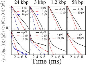
Time correlation functions in dsDNA tethers of varying contour length at different forces. Time correlation functions were measured along the y axis (〈_y_2+(0) y+(t)〉, 〈_y_−(0) _y_−(t)〉) and normalized by the variances (〈_y_2+〉, 〈_y_2+〉). (Upper panels) Correlation function for fluctuations of the center of mass. The correlation function shows a simple exponential decay as expected for a single-component noise. The correlation function changes with force due to trap nonlinearity (change in trap stiffness) but does not show dependence on the length of the tether. (Lower panels) Correlation function for the distance between the centers of the beads. These correlation functions show a double-exponential behavior (Fig. 6) which denotes the presence of two relaxational processes. Data for 58 bp and 1.2 kbp DNA tethers are not shown at 16 pN as these experiments were carried out on tethers with an inserted hairpin which unfolds at ∼14 pN (4), and the released ssDNA would affect the stiffness measurement.
Whereas the correlation function for the center of mass shows a single-exponential behavior (upper panels), the differential coordinate displays a double-exponential behavior that derives from the coupling of fluctuations (lower panels). This is the expected phenomenology for tether misalignment, which is the dominant effect in our setup. On the contrary, in the case of trap misalignment, both the differential and center-of-mass coordinates would be affected. According to Eqs. 27 and 28 and neglecting the trap stiffness with respect to the molecular stiffness (k m ≫ k y, k z; f/_r_0 ≫ k z), we have that, in the presence of tether misalignment, the variance of the differential coordinate _y_− changes to
| 〈y−2〉≃kBT2km(1+(r0kmf−1)ϵ2). | (42) |
|---|
As the value of ε is not known, the derivation of the molecular stiffness cannot be performed on the basis of variance analysis. Fortunately, as already noted in Meiners and Quake (5), the decay rate of fluctuations in the optical plane ω+ is much bigger than that of fluctuations along the optical axis _ω_−. The correlation function for _y_− (derived in the Supporting Material) reads as
| 〈y−(0)y−(t)〉=(1−ϵ2)e−2ω+t2km+ϵ2r0e−2ω−t2f, | (43) |
|---|
and the molecular stiffness can still be recovered by selecting the amplitude of the fast decaying component of the correlation function (Fig. 6). Using this data analysis technique, we measured the force-dependent stiffness of the different tethers (Fig. 7).
Figure 6.
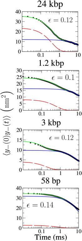
Fast and slow components of the correlation function of the differential coordinate. Double-exponential fits to 〈_y_−(0), _y_−(t)〉 in semi-log plot. (Dots) For experimental data, the continuous fair curve superimposed on the data shows a double-exponential fit to the measured data. (Dark solid curves) Fast and slow components of the double-exponential fit. Every plot reports the value of ε, the coupling strength as obtained from Eq. 42. As the molecules get shorter, the relative weight of slow fluctuations increases, indicating a stronger coupling.
Figure 7.
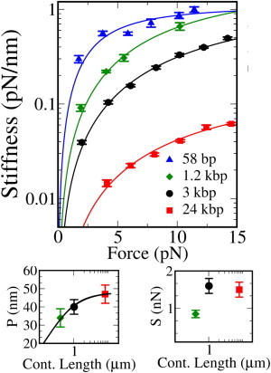
Measurement of the molecular stiffness. (Main figure) Measured molecular stiffness for four tethers 58 bp (triangles), 1.2 kbp (diamonds), 3 kbp (squares), and 24 kbp (circles), as a function of the mean force along the tether. (Symbols) For measured quantities, data from at least three different molecules have been averaged in the four cases. (Solid lines) EWLC fit to the data (main text). The Marko-Siggia approximation is not valid in the case of the shortest (58 bp) molecule. In this case, the fit is only meant to compare the results obtained in the DTOT with those reported in Forns et al. (4) obtained in a STOT. The fit results are shown in Table 1. (Upper-right panel) Comparison of the measured persistence length (P) of the three longer tethers to the empirical scaling law proposed by Seol et al. (14) in Eq. 45 (solid line). Fit parameters are discussed in the main text. (Lower-right panel) Measured stretch modulus for the three longer tethers. Errors in P and S values are standard deviation over at least three different molecules.
The nonlinear elasticity of dsDNA is usually modeled with the wormlike chain (WLC) model. When a contribution for enthalpic stretching and overwinding (12) is added, the so-called extensible WLC (EWLC) (13) model is obtained. The Marko-Siggia approximation formula for the force-dependent stiffness of an EWLC is
| km(f)=1ℓ0(14kBTP(1f)3/2+1S)−1, | (44) |
|---|
where P is the persistence length of the polymer, ℓ0 is its contour length, and S is the stretch modulus. This approximation is valid for molecules whose contour length is larger than the persistence length, (_l_0 < P) (13). The EWLC model was fitted to the data, letting the persistence length P and the stretch modulus S vary. Fit results are shown in Table 1. In all cases, the results are compatible with the existing literature, although they were derived in a different force range. In particular, the 3-kbp molecule shows a decrease in persistence length, which is compatible with theoretical predictions based on finite-size effects as recently shown in Seol et al. (14). Data for the 1.2-kbp and 58-bp tethers are instead consistent with measurements performed in an STOT (4). In principle, 58-bp data should not be fitted with the Marko-Siggia approximation (_l_0 < P), and a semiflexible rod model is required. Nevertheless, we decided to include the results for such short tether in Fig. 7 to stress the agreement between our dual-trap measurements and those reported in Forns et al. (4) for a STOT.
Table 1.
Persistence length and stretch modulus for different dsDNA tethers
| Molecule | Fit results | |
|---|---|---|
| P (nm) | S (pN) | |
| 24 kbp | 48 ± 5 | 1400 ± 300 |
| 3 kbp | 39 ± 4 | 1800 ± 400 |
| 1.2 kbp | 34 ± 5 | 850 ± 100 |
| 58 bp | 1.4 ± 0.8 | 20 ± 2 |
Several recent measurements on dsDNA suggest a strong reduction of the persistence length as the contour length of the molecule decreases. This could be the result of scale-dependent DNA elasticity, as already found in microtubules (15), or a finite-size effect due to the boundary conditions (14). Here we carry out persistence-length measurements in the highly stretched regime (2–15 pN), i.e., when the molecule is almost fully stretched and the enthalpic contribution is important (13,16). In this regime and in contrast to low force measurements (14,17,18), excluded volume effects between the trapped beads are negligible. Moreover, the effect of fluctuating boundary conditions on the force-extension curve should become less and less relevant as f R b grows, with f the mean tension along the tether and R b the bead radius (≃2 _μ_m in our experiments). Seol et al. (14) propose a phenomenological scaling equation:
We fitted such empirical formula to our persistence-length measurements, leaving out the shortest tether whose persistence length cannot be correctly measured using the Marko-Siggia approximation. The parameters obtained from the fit are _P_∞ = 49 ± 2 nm, in accordance with those measured in Seol et al. (14) and a = 4 ± 1, which is bigger than the value (2.78) measured in Seol et al. (14) and later confirmed in Chen et al. (17). It must be stressed that our experiments are performed in a dumbbell configuration, whereas both Seol et al. (14) and Chen et al. (17) have one of the ends of the molecule attached to a surface, and the boundary conditions imposed on the molecule are different in the two cases. The finite size WLC theory (14) does indeed predict a faster decrease of the effective persistence length with the contour length in the dumbbell configuration.
Conclusions
Misalignment effects may affect any optical-tweezers setup and the effect of a small misalignment can be enhanced by the large difference in stiffness between fluctuations along the pulling direction and along the optical axis. For analyzing these effects, we have provided tools to estimate their relevance; we have shown that trap and tether misalignments lead to different coupling structures and explained how to include couplings in the data analysis. When misalignment is negligible, it is possible to measure the stiffnesses of traps and tether from a straightforward analysis of the measured variance of force (or position) signals. This technique may be used as a calibration technique, valid beyond the linear trap region, in any DTOT. Otherwise, it is possible to include misalignment effects in data analysis. Such techniques have been used to measure the stiffness of dsDNA tethers of three different lengths, from 24 kbp to 1200 bp. The stiffness was interpreted in the framework of the EWLC model and we confirmed the decrease in apparent persistence length previously reported in Seol et al. (14) and Chen et al. (17), although our measurements were performed in a wider force range and with a different setup.
Acknowledgments
It is a pleasure to thank Sergio Ciliberto, Matthias Rief, Jeff Moffitt and Michael Woodside for useful discussions.
MR is supported by HFSP Grant No. RGP55-2008. FR is supported by MICINN FIS2010-19342, HFSP Grant No. RGP55-2008, and ICREA Academia grants.
Supporting Material
Document S1. The mathematical derivation of some of the results discussed in the main text
References
- 1.Meiners J.C., Quake S.R. FemtoNewton force spectroscopy of single extended DNA molecules. Phys. Rev. Lett. 2000;84:5014–5017. doi: 10.1103/PhysRevLett.84.5014. [DOI] [PubMed] [Google Scholar]
- 2.Smith S.B., Cui Y., Bustamante C. Optical-trap force transducer that operates by direct measurement of light momentum. Methods Enzymol. 2003;361:134–162. doi: 10.1016/s0076-6879(03)61009-8. [DOI] [PubMed] [Google Scholar]
- 3.Huguet J.M., Bizarro C.V., Ritort F. Single-molecule derivation of salt dependent base-pair free energies in DNA. Proc. Natl. Acad. Sci. USA. 2010;107:15431–15436. doi: 10.1073/pnas.1001454107. [DOI] [PMC free article] [PubMed] [Google Scholar]
- 4.Forns N., de Lorenzo S., Ritort F. Improving signal/noise resolution in single-molecule experiments using molecular constructs with short handles. Biophys. J. 2011;100:1765–1774. doi: 10.1016/j.bpj.2011.01.071. [DOI] [PMC free article] [PubMed] [Google Scholar]
- 5.Meiners J.C., Quake S.R. Direct measurement of hydrodynamic cross correlations between two particles in an external potential. Phys. Rev. Lett. 1999;82:2211–2214. [Google Scholar]
- 6.Bustamante C., Chemla Y., Moffitt J. High-resolution dual-trap optical tweezers with differential detection: alignment of instrument components. Cold Spring Harbor Protocols. 2009 doi: 10.1101/pdb.ip76. [DOI] [PubMed] [Google Scholar]
- 7.Gebhardt J.C., Bornschlögl T., Rief M. Full distance-resolved folding energy landscape of one single protein molecule. Proc. Natl. Acad. Sci. USA. 2010;107:2013–2018. doi: 10.1073/pnas.0909854107. [DOI] [PMC free article] [PubMed] [Google Scholar]
- 8.Comstock M.J., Ha T., Chemla Y.R. Ultrahigh-resolution optical trap with single-fluorophore sensitivity. Nat. Methods. 2011;8:335–340. doi: 10.1038/nmeth.1574. [DOI] [PMC free article] [PubMed] [Google Scholar]
- 9.Neuman K.C., Block S.M. Optical trapping. Rev. Sci. Instrum. 2004;75:2787–2809. doi: 10.1063/1.1785844. [DOI] [PMC free article] [PubMed] [Google Scholar]
- 10.Tolić-Nųrrelykke S., Schäffer E., Flyvbjerg H. Calibration of optical tweezers with positional detection in the back focal plane. Rev. Sci. Instrum. 2006;77:103101. [Google Scholar]
- 11.Jahnel M., Behrndt M., Grill S.W. Measuring the complete force field of an optical trap. Opt. Lett. 2011;36:1260–1262. doi: 10.1364/OL.36.001260. [DOI] [PubMed] [Google Scholar]
- 12.Gore J., Bryant Z., Bustamante C. DNA overwinds when stretched. Nature. 2006;442:836–839. doi: 10.1038/nature04974. [DOI] [PubMed] [Google Scholar]
- 13.Marko J., Siggia E. Stretching DNA. Macromolecules. 1995;28:8759–8770. [Google Scholar]
- 14.Seol Y., Li J., Betterton M.D. Elasticity of short DNA molecules: theory and experiment for contour lengths of 0.6–7 micrometers. Biophys. J. 2007;93:4360–4373. doi: 10.1529/biophysj.107.112995. [DOI] [PMC free article] [PubMed] [Google Scholar]
- 15.Pampaloni F., Lattanzi G., Florin E.L. Thermal fluctuations of grafted microtubules provide evidence of a length-dependent persistence length. Proc. Natl. Acad. Sci. USA. 2006;103:10248–10253. doi: 10.1073/pnas.0603931103. [DOI] [PMC free article] [PubMed] [Google Scholar]
- 16.Marko J. Stretching must twist DNA. Euro. Phys. Lett. 1997;38:183. [Google Scholar]
- 17.Chen Y.F., Wilson D.P., Meiners J.C. Entropic boundary effects on the elasticity of short DNA molecules. Phys. Rev. E Stat. Nonlin. Soft Matter Phys. 2009;80:020903. doi: 10.1103/PhysRevE.80.020903. [DOI] [PubMed] [Google Scholar]
- 18.Chen Y.F., Blab G.A., Meiners J.C. Stretching submicron biomolecules with constant-force axial optical tweezers. Biophys. J. 2009;96:4701–4708. doi: 10.1016/j.bpj.2009.03.009. [DOI] [PMC free article] [PubMed] [Google Scholar]
- 19.Smith S.B., Cui Y., Bustamante C. Overstretching B-DNA: the elastic response of individual double-stranded and single-stranded DNA molecules. Science. 1996;271:795–799. doi: 10.1126/science.271.5250.795. [DOI] [PubMed] [Google Scholar]
Associated Data
This section collects any data citations, data availability statements, or supplementary materials included in this article.
Supplementary Materials
Document S1. The mathematical derivation of some of the results discussed in the main text