A Perspective on Epistasis: Limits of Models Displaying No Main Effect (original) (raw)
Abstract
The completion of a draft sequence of the human genome and the promise of rapid single-nucleotide-polymorphism–genotyping technologies have resulted in a call for the abandonment of linkage studies in favor of genome scans for association. However, there exists a large class of genetic models for which this approach will fail: purely epistatic models with no additive or dominance variation at any of the susceptibility loci. As a result, traditional association methods (such as case/control, measured genotype, and transmission/disequilibrium test [TDT]) will have no power if the loci are examined individually. In this article, we examine this class of models, delimiting the range of genetic determination and recurrence risks for two-, three-, and four-locus purely epistatic models. Our study reveals that these models, although giving rise to no additive or dominance variation, do give rise to increased allele sharing between affected sibs. Thus, a genome scan for linkage could detect genomic subregions harboring susceptibility loci. We also discuss some simple multilocus extensions of single-locus analysis methods, including a conditional form of the TDT.
Introduction
A quarter century ago, the advent of recombinant-DNA technology spurred what can arguably be called the “golden age of human linkage studies.” The availability of a large number of new DNA markers that could be typed directly (e.g., RFLPs, VNTRs, and microsatellites), coupled with major advances in computer software and hardware, meant that the mapping of genes that are individually sufficient to cause human disease rested on little more than the collection of an adequate sample of segregating families.
The approach is straightforward. A genome scan using 300–400 short-sequence tandem-repeat markers reveals a single linkage signal. Additional markers are added to saturate this chromosomal region. Subsequent identification of recombinants delimits the genomic segment containing the disease-causing gene. A search is then initiated to identify all variants in the region (insertions, deletions, single-nucleotide polymorphisms [SNPs], repeat polymorphisms, etc.), and these, in turn, are tested for cosegregation with the disease, usually in the same families in which the original linkage signal was found. Once the genetic lesion is identified, functional analysis is used to clarify how the lesion alters disease susceptibility.
This idealized scenario is not intended to trivialize the hard work needed to successfully complete each step. Ten years, for instance, elapsed between the mapping of the locus responsible for Huntington disease to chromosome 4p (Gusella et al. 1983) and the subsequent identification of the expanded CAG repeat in the gene’s first exon (Huntington’s Disease Collaborative Research Group 1993). Nonetheless, a litany of disease genes that have been identified during the past 2 decades is ample testimony to this strategy’s success.
But what about complex diseases? Is it reasonable to suppose that an approach that must succeed in identifying fully penetrant Mendelian genes will also succeed for complex diseases? Most gene sleuths would answer yes—but would add the caveat that, since recombinants cannot be identified unambiguously, ancillary approaches are needed as well. Three approaches that often accompany linkage studies of complex diseases are (1) family-based association studies (Spielman et al. 1993), (2) case-control studies (Woolf 1955), and (3) measured genotype studies (Boerwinkle et al. 1986). All of these ancillary approaches tacitly assume that allelic variation in or around a particular susceptibility locus makes a measurable difference in the phenotype. The reasonableness of this assumption is so obvious that it is rarely explicitly stated.
If the advances wrought a generation ago by recombinant-DNA technology can be said to have revolutionized genetic research, we believe that the field is poised to experience an even greater revolution in the near future. Against the backdrop provided by the completion of a draft sequence of the human genome, it is reasonable to expect that both SNP and expression-microarray technologies will forever change how research in human genetics is pursued. Moreover, we believe that these new technologies will make the three ancillary strategies mentioned above all the more attractive to researchers—even to the point of supplanting traditional linkage analysis—for at least two reasons: first, it has been argued that linkage methods simply do not have the power to detect the small signals that can be expected under some disease models (Risch and Merikangas 1996); second, even when appropriate power can be obtained, multiplex pedigrees are substantially more expensive to gather than are a series of unrelated patients (for measured-genotype analyses), a series of patients and “matched” unaffected subjects (for comparison with patients in case-control studies), or parents and a single affected offspring (for family-based association studies).
The complex relationship between genotype and phenotype, however, may ultimately prove to be inadequately described by simply summing the modest effects from several contributing loci. Instead, the relationship may, as Sewell Wright (1923) argued, depend in a fundamental way on epistasis (i.e., the interaction between loci) and genotype × environment interaction. Indeed, it has been argued that epistatic interactions are a nearly universal component of the architecture of most common traits. Templeton (2000), for instance, has listed a number of phenotypes in which epistasis plays a large role. An example in insects is the abnormal-abdomen phenotype in Drosophila mercatorum (DeSalle and Templeton 1986; Hollocher et al. 1992; Hollocher and Templeton 1994). In humans, variation in triglyceride levels can be explained, in part, by two sets of interactions: between ApoB and ApoE in females and between the ApoAI/CIII/AIV complex and low-density lipoprotein receptor in males (Nelson et al. 2001). Even the seemingly “simple” Mendelian trait of sickle-cell anemia is revealed to be greatly modified by epistatic interactions. Individuals with sickle-cell anemia who are homozygous for two polymorphisms near the Gγ locus (leading to the persistence of fetal hemoglobin) have only mild clinical symptoms (Odenheimer et al. 1983; Sing et al. 1985; el-Hazmi et al. 1992). Other human diseases that recently have been reported to exhibit epistatic interactions are Alzheimer disease (Zubenko et al. 2001) and breast cancer (Ritchie et al. 2001).
The main reason that most studies of complex human phenotypes fail to find evidence for epistatic interactions may simply be that commonly used designs and analytic methods inherently minimize or exclude the possibility of epistasis (Frankel and Schork 1996). Because the investment in new study designs and analytic methods may be high, we decided to examine the extent to which purely epistatic interactions (i.e., interactions between loci that do not display any single-locus effects) could account for phenotype.
In the present article, we explore a class of transmission models in which each contributing susceptibility locus has no phenotypic effect detectable by any of the three ancillary approaches listed above. For these epistatic models, the proper “unit of analysis” is not the allelic variation at a single locus but, rather, is the multilocus genotype. We show that, in spite of the undetectability of the contributing loci by the three ancillary approaches, these models can result in both high heritability and substantial increases in recurrence risk to a proband’s relatives. In addition, we show that the increased allele sharing engendered by these models can be sufficient to allow the detection of the contributing loci by linkage.
Since the space of epistatic models whose contributing loci display no main effects is very large, we elected to map an extreme envelope of these models. Our approach is similar in spirit to the determination of the limits of the two-allele single-locus model with any arbitrary penetrance vector (Suarez et al. 1976) and to its generalization to multiple loci (Craddock et al. 1995). Although there is no doubt that many phenotypes result from the epistatic interaction of two or more loci, it is unknown how often phenotypes correspond to the limiting conditions considered here.
Models
Consider a dichotomous qualitative trait (e.g., “affected” vs. “unaffected” phenotype) determined by L biallelic loci. We examine the extent to which affection status can be genetically determined (i.e., “broad sense” heritability) in models for which the marginal penetrance for each of the three genotypes is equal to K, the population prevalence of the disease, for each of the contributing loci. In what follows, we assume that all disease-susceptibility loci are in Hardy-Weinberg equilibrium and that alleles at different susceptibility loci are in linkage equilibrium.
Two-Locus Models
Let the alleles from locus A be denoted “_A_” and “_a,_” and let those from locus B be denoted “_B_” and “_b._” At locus A, let AA be genotype 1, Aa be genotype 2, and aa be genotype 3, and let the genotypes at locus B be defined correspondingly. Let p A be the allele frequency of A, and let p B be the allele frequency of B. Let f ij be the disease penetrance for the genotype consisting of genotype i at locus A and genotype j at locus B. Let M Ai be the marginal penetrance for genotype i at locus A, and let M Bj be the marginal penetrance for genotype j at locus B.
The relationship between these variables is given by the formulae
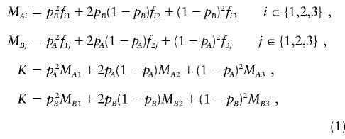
and is commonly represented by the penetrance table seen in table 1. For all of the genetic variation to be epistatic, a two-locus model must also satisfy

Table 1.
Penetrances for a Generic Biallelic Two-Locus Model
| Penetrance of Genotype | ||||
|---|---|---|---|---|
| Genotype | BB | Bb | bb | Marginal Penetrance |
| AA | _f_11 | _f_12 | _f_13 | M _A_1 |
| Aa | _f_21 | f22 | _f_23 | M _A_2 |
| aa | _f_31 | f32 | _f_33 | M _A_3 |
| Marginal penetrance | M _B_1 | M _B_2 | M _B_3 | K |
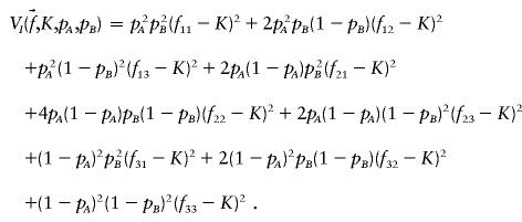
To explore the space of penetrance models that satisfy formulae (1) and formula (2), we varied K, p A , and p B . For each set of parameter values, we searched for a penetrance model that would maximize the proportion of variation attributable to genotype. The total variance of the dichotomous phenotype in the population is V T(K)=K(1-K). For models satisfying formulae (1) and formula (2), all of the variation attributable to genotype is epistatic. This variation, V I , is given by the following formula
Thus, for fixed K, p A , and p B , maximizing the broad heritability (_h_2=V I/V T) under the constraint represented by formula (2) is equivalent to the maximizing of V I.
The constraints represented by formulae (1) imply that, for fixed K, p A , and p B , the remaining five penetrances can be written as linear combinations of the four corner penetrances: _f_11, _f_13, _f_31, and _f_33. Therefore, the set of f ij satisfying formulae (1) and formula (2) forms a four-dimensional polyhedral subset of the nine-dimensional unit hypercube, Π9_i_=1[0,1]. Our goal is to maximize V I over this polyhedron. A linear transformation converts this problem to the problem of maximizing the distance between a fixed point in the interior of the polyhedron and other points in the polyhedron. Therefore, one of the vertices of the polyhedron must correspond to a model generating the maximum heritability. Determining the vertices of the polyhedron is a linear-algebra problem that can, in theory, be solved explicitly for any fixed values of our parameters. Because of the number of constraints involved, we used the cdd+ program (see the “cdd and cddplus Homepage”), which implements the “double description method” (Motzkin et al. 1953) to find the vertices of the polyhedra of two-locus purely epistatic models.
Table 2 lists estimated maximum heritabilities for various combinations of K, p A , and p B . For most K, the greatest heritability was found when p _A_=p _B_=0.5.
Table 2.
Maximum Heritability in Purely Epistatic Two-Locus Models
| K | p A | p B | V I | _h_2 |
|---|---|---|---|---|
| .50 | .5 | .5 | .2500 | 1.000 |
| .4 | .2325 | .930 | ||
| .3 | .2411 | .964 | ||
| .2 | .1406 | .563 | ||
| .1 | .0422 | .169 | ||
| .4 | .4 | .2200 | .880 | |
| .3 | .2256 | .902 | ||
| .2 | .1308 | .523 | ||
| .1 | .0545 | .218 | ||
| .3 | .3 | .2355 | .942 | |
| .2 | .1356 | .542 | ||
| .1 | .0566 | .226 | ||
| .2 | .2 | .0791 | .316 | |
| .1 | .0330 | .132 | ||
| .40 | .5 | .5 | .1700 | .708 |
| .4 | .1592 | .663 | ||
| .3 | .1589 | .662 | ||
| .2 | .1012 | .467 | ||
| .1 | .0422 | .176 | ||
| .4 | .4 | .1744 | .727 | |
| .3 | .1610 | .671 | ||
| .2 | .1181 | .492 | ||
| .1 | .0493 | .205 | ||
| .3 | .3 | .1673 | .697 | |
| .2 | .1243 | .518 | ||
| .1 | .0518 | .216 | ||
| .2 | .2 | .1139 | .475 | |
| .1 | .0475 | .198 | ||
| .20 | .5 | .5 | .0800 | .500 |
| .4 | .0555 | .347 | ||
| .3 | .0472 | .295 | ||
| .2 | .0362 | .226 | ||
| .1 | .0281 | .276 | ||
| .4 | .4 | .0615 | .384 | |
| .3 | .0486 | .292 | ||
| .2 | .0400 | .250 | ||
| .1 | .0292 | .182 | ||
| .3 | .3 | .0449 | .281 | |
| .2 | .0311 | .194 | ||
| .1 | .0185 | .116 | ||
| .2 | .2 | .0409 | .256 | |
| .1 | .0199 | .124 | ||
| .10 | .5 | .5 | .0200 | .222 |
| .4 | .0139 | .154 | ||
| .3 | .0118 | .131 | ||
| .2 | .0091 | .101 | ||
| .1 | .0070 | .078 | ||
| .4 | .4 | .0200 | .222 | |
| .3 | .0145 | .161 | ||
| .2 | .0104 | .116 | ||
| .1 | .0089 | .099 | ||
| .3 | .3 | .0178 | .198 | |
| .2 | .0097 | .108 | ||
| .1 | .0054 | .060 | ||
| .2 | .2 | .0113 | .126 | |
| .1 | .0050 | .056 |
An alternative visualization tool is to vary K while keeping p A and p B constant. Using cdd+, we were able to parameterize the vertices of the space of two-locus purely epistatic models when p _A_=p _B_=0.5, in terms of K. The range of K examined was (0, 1/2] because the maximum heritabilities are necessarily symmetric about _K_= 1/2. We found that there are 7 vertices when _K_∈(0, 1/4] and that there are 25 vertices when _K_∈( 1/4, 1/2]. The curves corresponding to the maximum heritabilities are described by the following formulae:
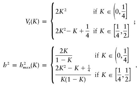
These maxima can be achieved using the penetrances given in table 3, for _K_∈(0, 1/4], and the penetrances given in table 4, for _K_∈[ 1/4, 1/2].
Table 3.
Two-Locus Penetrances Yielding Maximum **h**2 for _K_∈(0, 1/4]
| Penetrance of Genotype | |||
|---|---|---|---|
| Genotype | BB | Bb | bb |
| AA | 0 | 0 | 4_K_ |
| Aa | 0 | 2_K_ | 0 |
| aa | 4_K_ | 0 | 0 |
Table 4.
Two-Locus Penetrances Yielding Maximum **h**2 for 
| Penetrance of Genotype | |||
|---|---|---|---|
| Genotype | BB | Bb | bb |
| AA | 4_K_-1 | 0 | 1 |
| Aa | 0 | 2_K_ | 0 |
| aa | 1 | 0 | 4_K_-1 |
A plot of population prevalence versus maximum heritability is shown in figure 1. This graph also contains a plot of K versus total variance and of K versus maximum epistatic variance.
Figure 1.

Limits of two-locus, biallelic, purely epistatic (i.e., V _A_=V _D_=0 at each locus) models, with all alleles equally frequent. The bottom curve represents the maximum variance due to genotype (i.e., V I), the middle curve represents the total variance as a function of disease prevalence (i.e., V _T_=K(1-K)), and the top curve represents the maximum proportion of variance attributable to genotype (i.e., _h_2=V I/V T).
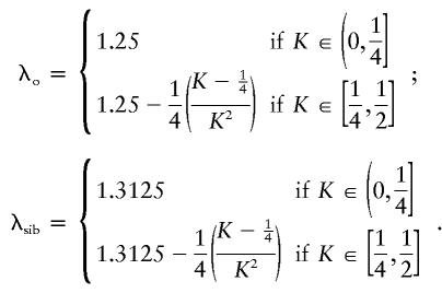
Figure 1 illustrates that there exist two-locus models with no marginal genotypic effect at either locus but in which genotype nonetheless accounts for a large portion of the population variance. Although the heritability can be high in these models, the constraints that eliminate any marginal gene effects keep the recurrence risks modest. In the manner described by Risch (1990), the relative risks to offspring (λo) and to sibs (λsib) of an affected individual can be computed from the parent-offspring covariance and the sibling covariance, respectively. To compute these covariances, we used the variance components as derived by Tiwari and Elston (1997). We found that, for the models in tables 3 and 4, λo and λsib are given by the following formulae:
Three-Locus Models
Although the vertices of the polyhedra of purely epistatic models can, in theory, always be found, in practice it proved computationally impractical, for many three-locus parameter sets. These sets often involve several thousand vertices. We found that a slight perturbation in K could lead to a 20,000-fold increase in computing time.
For this reason, we estimated the maxima for three-locus models by using the nonlinear maximization methods implemented in the SAS Institute (1995) procedure PROC NLP. Because this method estimates local rather than global maxima, we used 1,000 random seeds for each parameter set, choosing the highest resulting epistatic variance as our approximation of the true maximum. We verified this approach on two-locus models, finding the true maximum at each of 100 points.
Three-locus models produce a dramatic increase in the maximum proportion of variation explainable by genotype, as can be seen in figure 2. For the three-locus case, we again have found specific models that closely fit the numerically derived maxima plotted as dots in figure 2, where the curves generated by these models are drawn as a line beneath the dots. The fact that we could find models with V I at least as high as the iterative estimates for each K indicates that rounding errors from SAS are not likely to cause substantial overestimation of the maximum heritability. In fact, for a few points near _K_=0.4 and _K_=0.46, the empirical estimate slightly underestimated the true maximum. Formulae for the curves in figure 2 can be found in the Appendix.
Figure 2.

Limits of three-locus, biallelic, purely epistatic (i.e., V _A_=V _D_=0 at each locus) models, with all alleles equally frequent. The bottom curve represents the approximate maximum variance due to genotype (i.e., V I), estimated by an iterative maximization algorithm from the SAS Institute (1995), the middle curve represents the total variance (i.e., V _T_=K(1-K)) as a function of disease prevalence, and the top curve represents the values for _h_2 that we have found for particular models; the dots on the top curve are the maximum proportion of variance attributable to genotype (i.e., _h_2=V I/V T), estimated by the iterative maximization method.
The maximum possible heritability in models with no single-locus additive or dominance variance is increased dramatically in three-locus models compared with two-locus models. For heritability to reach 90%, two-locus models require a disease prevalence >47%, whereas three-locus models can be completely genetic for prevalences as low as 25%. Furthermore, for _K_=0.05–0.10, a range that includes the prevalences of many complex diseases, three-locus models can generate heritabilities of 35%–55%. In contrast, purely epistatic two-locus models can only generate 10%–22% heritability.
Three-locus models can also give rise to higher relative risks than are possible in corresponding two-locus models. Three-locus penetrance models maximizing heritability at the low end of disease prevalence (_K_∈(0, 1/16]) are parameterized in table 5. These models correspond to λ_sib_=2.125 (again computed by use of components of variance that are derived by Tiwari and Elston [1997]). In contrast, the highest λsib possible for two-locus epistatic models is 1.3125.
Table 5.
Three-Locus Penetrances Yielding Maximum **h**2 for _K_∈(0, 1/16]
| Penetrance of Genotype | |||||||||
|---|---|---|---|---|---|---|---|---|---|
| CC | Cc | cc | |||||||
| Genotype | BB | Bb | bb | BB | Bb | bb | BB | Bb | bb |
| AA | 0 | 0 | 16_K_ | 0 | 0 | 0 | 0 | 0 | 0 |
| Aa | 0 | 0 | 0 | 0 | 4_K_ | 0 | 0 | 0 | 0 |
| aa | 0 | 0 | 0 | 0 | 0 | 0 | 16_K_ | 0 | 0 |
Because none of the alleles in these models have any marginal effect on disease susceptibility, the disease would not cause selection pressure on allele frequency at any of the loci. Nonetheless, genetic drift, mutation, and selection pressure from factors other than the disease in question are likely to cause the allele frequencies to be perturbed from 50%:50%. Figure 3 illustrates the effect that unbalanced allele frequencies have on these models. In this figure, p i denotes the frequency of the less common allele at locus i. (This should not be interpreted as the “disease allele” frequency. In these models, there are no “disease alleles,” only “disease genotypes.”) Although, in models with these unbalanced allele frequencies (i.e., 40%:60%, 20%:80%, and 20%:80%), the total variance attributable to genotype is smaller than that in models in which all alleles are equally frequent, a sizable portion of the variation can still be explained by genotype.
Figure 3.

Limits of three-locus, biallelic, purely epistatic (i.e., V _A_=V _D_=0 at each locus) models. The bottom curve represents the estimated maximum variance due to genotype (i.e., V I), the middle curve represents the total variance (i.e., V _T_=K(1-K)) as a function of disease prevalence, and the top curve represents the estimated maximum proportion of variance attributable to genotype (i.e., _h_2=V I/V T).
Four-Locus Models
Figure 4 illustrates the estimated maximum heritabilities possible for models involving four interacting loci. The maximum heritability remains >90% for prevalences >12%, and maximum heritability is not much less than 50% unless prevalence is <2%. Furthermore, for prevalences of 0%–2%, the maximum heritability possible with four loci is approximately four times as high as that for models involving three loci. Some of the jaggedness seen in figure 4 may be attributable to the fact that points for K are plotted in increments of 0.0025 and that only 1,000 iterations were used for each point. We have observed that using too few iterations can considerably underestimate the maximum heritability.
Figure 4.

Limits of four-locus, biallelic, purely epistatic (i.e., V _A_=V _D_=0 at each locus) models, with all alleles equally frequent. The bottom curve represents the estimated maximum variance due to genotype (i.e., V I), the middle curve represents the total variance (i.e., V _T_=K(1-K) as a function of disease prevalence, and the top curve represents the estimated maximum proportion of variance attributable to genotype (i.e., _h_2=V I/V T).
As before, the addition of a locus corresponds to an increase in recurrence risk to relatives. At the low end of disease prevalence (K<0.0156), λsib can reach 2.609 (calculated as above), in contrast to λ_sib_=2.125 for three-locus models and λ_sib_=1.3125 for two-locus models.
Also, when the allele frequencies are perturbed from 50%:50%, the maximum-heritability curves for four-locus models appear to be more stable than those for three-locus models. This can be seen by comparing figure 4 with figure 5. Figure 5 displays results from four-locus models in which the frequencies of the less common alleles are 20% at locus A, 30% at locus B, 40% at locus C, and 50% at locus D. Maximum heritability remains >95% for disease prevalences >16% and does not fall to <50% unless the disease prevalence is <4%.
Figure 5.

Limits of four-locus, biallelic, purely epistatic (i.e., V _A_=V _D_=0 at each locus) models. The bottom curve represents the estimated maximum variance due to genotype (i.e., V I), the middle curve represents the total variance (i.e., V _T_=K(1-K)) as a function of disease prevalence, and the top curve represents the estimated maximum proportion of variance attributable to genotype (i.e., _h_2=V I/V T).
Detection of Epistatically Interacting Loci
Association
By design, the models described here have equal marginal penetrances for all single-locus genotypes. Because of this, it is obvious that a qualitative measured-genotype analysis of a single locus (analogous to the quantitative measured genotype described by Boerwinkle et al. [1986]) could not detect any of the contributing loci. Furthermore, the equality of the marginal penetrances implies that cases and controls have identical allele distributions at the contributing loci. Thus, a case-control study examining one locus at a time would also fail to detect the contributing loci.
A transmission/disequilibrium test (TDT [Spielman et al. 1993]) study examining a single locus at a time would also fail to detect the contributing loci, but the reasons may seem less obvious. Within particular families, heterozygous parents would preferentially transmit allele A to their affected offspring; however, in a similar proportion of families, heterozygous parents would preferentially transmit allele a to affected offspring. The TDT, in common with other association analyses, keeps track of the particular “at risk” allele that is either differentially present in affected individuals or preferentially transmitted to affected offspring. Thus, the evidence from families transmitting allele A will “cancel out” the evidence from families transmitting allele a. As a result, under these purely epistatic models, the TDT statistic for the contributing loci will be equivalent to those for “neutral” loci.
Since it is impossible to detect these loci by use of a locus-by-locus genome scan for association, one might consider a scan assessing two or more loci at a time. Estimates of the number of SNPs required for a whole-genome scan range from as many as 500,000 (Kruglyak 1999) to as few as 30,000 (Collins et al. 1999). To examine all two-way interactions for even the smaller number would require ∼450 million tests; to examine all three-way interactions would require ∼4.5 trillion tests. These are nontrivial computational tasks, not to mention the statistical problem of correcting for multiple tests.
The fact that the number of tests involved in examining the interactions grows as a polynomial in the number of loci suggests that successful analyses of interactions will depend on a method of selecting a limited number of candidate loci for consideration. Fortunately, for the class of models discussed in the present article, linkage analysis is often able to detect increased allele sharing at loci that epistatically contribute to the affected phenotype.
Linkage
Although the purely epistatic models discussed here do not give rise to different allele frequencies in cases and controls, they do give rise to excess allele sharing among affected sibs. Because these epistatic models have no “disease alleles” (only “disease genotypes”), the allele that is shared excessively among affected sibs varies depending on the mating type of the parents. However, in contrast to association analyses, if half of the families in a linkage analysis show increased sharing for allele A at locus A and the other half show increased sharing for allele a, then, for the combined sample, the linkage statistic at locus A is higher than that in either subsample. Because the linkage statistic from each family is not tied to a specific allele, the evidence for linkage from families segregating for different alleles accumulates rather than cancels. Consider, for instance, a collection of affected sib pairs with a disease that conforms to the two-locus model represented in table 3. Thirty-five of the possible 45 parental mating types are capable of segregating an affected child, and 28 of these mating types give rise to sib pairs with increased allele sharing at locus A, locus B, or both. Indeed, at each locus the expected proportion of alleles shared identical by descent is 4/7 (calculations not shown), regardless of the value of K. Hence, regions containing both loci are detectable by linkage analysis, provided that the sample size is adequate.
Analysis of Candidate Loci
Once a limited number of candidate loci are selected, it is feasible to examine the candidates for interactions. We note that the number of tests necessary to evaluate all two-, three-, and four-way interactions, for 30–60 candidate loci, has a range similar to the number of tests suggested for a single genomewide association scan using SNPs (Collins et al. 1999; Kruglyak 1999). Thus, although searching for two-, three-, four-, or _n_-way interactions among all the markers in a genome scan would not be practicable, a candidate-locus approach based on a genome scan for linkage may be.
Deriving appropriate and powerful methods to detect epistatic interactions remains a matter for further study. However, several straightforward methods are immediately available, and some more-elaborate methods are already in the literature.
Three Elementary Multilocus Methods
Cases only
The most straightforward multilocus analysis of cases-only data is a χ2 test of independent segregation for the loci. An analysis of data from the two-locus models described in table 3, for instance, yields an expected test statistic ⩾2_N,_ where N is the number of cases. This is a consequence of the fact that the expected value of the square of a random variable is at least as great as the square of the expected value of the variable. Under the null hypothesis of independent segregation, this statistic would be distributed as a χ2 with 4 df.
Case-control
A second approach is a multilocus case-control analysis. One method for doing this would be to compare the distribution of cases among the 3_L_ genotypes, where L is the number of biallelic loci being simultaneously examined, versus the distribution of controls.
In this analysis, a sample of N cases and N unrelated controls drawn from a population modeled by table 3 will, again, yield an expected χ2 statistic ⩾2_N._ However, the degrees of freedom under the null hypothesis are now 8. Moreover, compared to a cases-only strategy, the inclusion of unrelated controls will add to the cost of genotyping. In addition, for diseases with a variable age at onset, the inclusion of controls who will eventually develop the disease will compromise power.
Conditional TDT
Unrecognized population admixture can lead to false positives in both cases-only methods and case-control methods. The TDT was created to address this problem.
A conditional TDT is one possible way to address the same issue in a multilocus setting. For this, a sample of N trios is stratified by the genotype of the offspring at one (or more) of the candidate loci. A TDT analysis is then performed at another candidate locus, for each stratum of the data. The P values from the individual TDTs are then combined, by use of Fisher’s (1932) statistic (S_=-2Σ_m i_=1_ln(p i), where p i is the TDT P value corresponding to the i_th stratum of the data). Under the null hypothesis, S has a χ2 distribution with 2_m df, where m is the number of strata.
Consider, again, the model represented in table 3. When we condition on locus A, the trios with AA offspring would yield an expected χ2 statistic of N/4 if a TDT analysis were performed at locus B, the trios with aa offspring would yield the same expected χ2 statistic, and the trios with Aa offspring yield an expected χ2 statistic of 1, independent of sample size. The Fisher statistic in this case would be tested against a χ2 distribution with 6 df.
In the absence of population admixture, the conditional TDT (as well as the traditional TDT) is less powerful than a cases-only strategy or a case-control strategy. Furthermore, a TDT-type analysis comes at the additional cost of requiring a threefold increase in genotyping (i.e., two parents and the affected offspring), compared to the cases-only strategy.
Other methods
We do not claim that the methods described above are optimal in power; and they certainly are not exhaustive. They are simple to apply, however, and can be used to test any number of loci, for simultaneous interactions.
Other published multilocus analysis methods relying on association include the marker-association-sequence χ2, or “MASC,” method applied to two loci (Dizier et al. 1994). A method similar to the conditional TDT is the generalized TDT (Rice et al. 1995), if the genotypes at auxiliary loci are used as covariates. Nelson et al. (2001) used a combinatorial method for identifying the multilocus genotypes contributing to variation in serum triglyceride levels. Ritchie et al. (2001) used a related data-reduction technique to identify a four-locus risk factor for breast cancer.
Two-locus linkage methods include a sib-pair analysis (Dizier and Clerget-Darpoux 1986), a two-locus LOD-score method (Lathrop and Ott 1990; Schork et al. 1993), and a two-locus version of the maximum-LOD-score method (Cordell et al 1995).
Discussion
We have seen that, if the true genetic model underlying a disease is purely epistatic, with no additive or dominance variation at any of the susceptibility loci, then association methods analyzing one locus at a time will have no power to detect the loci. Nonetheless, linkage methods will have power and so might allow the detection of the susceptibility loci.
The models used to demonstrate these facts are boundary cases. They represent extreme limits in terms of two parameters: the marginal deviation is zero and, given that constraint, the heritability is at its maximum value. For any disease prevalence and for any allele-frequency distribution, merely relaxing the maximum heritability condition leads to infinitely many models that still display no single-locus marginal effect but that, nonetheless, may appear more “natural” in that they have nonzero penetrances for all genotypes. In fact, almost every purely epistatic model includes both incomplete penetrances and “phenocopies.”
Because few researchers specifically test for epistasis, it is difficult to gauge the extent to which purely epistatic interactions are involved in human disease. However, the chief importance of these results is not that purely epistatic models exist; rather, it lies in the implications that these results have for largely epistatic models with small marginal effects. Relaxing the condition of zero single-locus marginal deviation results in a much larger class of models, albeit a less mathematically tractable class. The heritabilities and λs found in the setting of zero marginal deviation are useful in providing lower bounds for the maximum values possible when marginal effects are small; in particular, although the models specifically discussed here are boundary cases, they imply that seemingly “natural” models can account for most of the variation in disease even if all the single-locus effects were to pass undetected.
Although we have only examined two-, three-, and four-locus models, the results lead us to two obvious extrapolations. First, we expect that, with a sufficient number of contributing loci, purely epistatic interactions could account for virtually all the variation in affection status for diseases with any prevalence. Second, models involving more loci could be associated with λs even greater than the 2.6 found for four-locus models.
Of course, there are subclasses of purely epistatic models (providing no marginal evidence for the involvement of any single locus) for which, in addition, no two, three, or _L_-1 loci jointly give evidence of involvement in the disorder. This leads to the concern that even assessment of all two-, three-, and (_L_-1)-way interactions among candidate loci may be insufficient for detection of the contributing loci.
This concern is ameliorated by the fact that such models are associated with lower heritabilities and much lower λ values than those of the models that we have examined. The restriction on maximum heritabilities in these models is most easily seen by examining _L_-locus models for which no collection of _L_-1 loci shows marginal deviations. The fact that all loci must pairwise satisfy the two-locus constraints implies that the maximum heritability in this case is theoretically bounded above by the values from the two-locus model. In fact, a check of three-locus models for which the two-locus marginal penetrances do not deviate from K (illustrated in fig. 6) shows that the true maximum heritability is even lower than the general upper bound.
Figure 6.

Comparison of maximum heritabilities for three-locus, purely epistatic models with (top curve) and without (bottom curve) two-locus interactions. The maximum heritabilities for two-locus, purely epistatic models (middle curve) are included as a reference.
The fact that λsib will diminish exponentially with the number of simultaneously hidden loci is a simple consequence of the formula relating the covariance between siblings and the components of variation. For an _L_-locus system, this is given by the following formula (Kempthorne 1957):
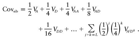
Thus, if M loci are “hidden,” Covsib cannot be greater than 2−M. For this reason, these models can make only a small contribution to λ.
Researchers of many complex diseases (including non–insulin-dependent diabetes mellitus, prostate cancer, and schizophrenia) face the conundrum of moderately heritable diseases for which locus-by-locus analyses have not accounted for the predicted genetic variance. The models discussed in the present article provide one possible explanation for this.
Had data been gathered for a disease that closely fitted one of the epistatic models considered here, it is likely that the linkage signals from the contributing loci would have been rejected as false positives. The impossibility of using locus-by-locus association analyses to either confirm or narrow the signal region would make it very easy to reject the true signals.
These considerations lead us to believe that, in situations in which heritability is moderate to high but in which locus-by-locus analyses do not account for the predicted genetic variance, it is worth pursuing a hypothesis of interacting loci near the linkage peaks. Even regions containing modest linkage signals may be good sources of candidate loci.
The epistatic models examined here were constructed so that none of the loci could be detected by case-control, measured-genotype, or TDT analyses of single loci. We found that a large fraction of the variation in affection status can be explained by such models, for a wide range of population prevalences and allele frequencies. Less extreme—and, therefore, more “natural”—models displaying small marginal effects can account for even more variation.
Since, for the class of epistatic models considered here, locus-by-locus linkage analyses do not suffer from the drawbacks of association analyses, we conclude that they will continue to prove useful even when dense SNP maps are available and rapid genotyping becomes less costly.
Acknowledgments
We would like to thank Drs. Saurabh Ghosh, Anthony Hinrichs, and John Rice for their help. This work was supported, in part, by U.S. Public Health Service grants MH14677, MH31302, and AA08403, by U.S. Army grant DAMD17-00-1-10108, and by an award from the Urological Research Foundation.
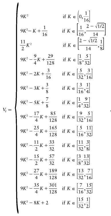
Appendix : Three-Locus Models
The formula below describes the estimated maximum-epistatic-variance curve for all models involving three loci. It was derived by use of specific models that we found by using our maximization search method. The third piece of the curve,
has a form different than that of the other pieces and has anomalous limits; nonetheless, checks of the vertices of the solution polyhedra for several values of K in and around this region confirm the estimated values.
Electronic-Database Information
The URL for data in this article is as follows:
- “cdd and cddplus Homepage,” http://www.ifor.math.ethz.ch/\~fukuda/cdd\_home/cdd.html [Google Scholar]
References
- Boerwinkle E, Chakraborty R, Sing CF (1986) The use of measured genotype information in the analysis of quantitative phenotypes in man. I. Models and analytical methods. Ann Hum Genet 50:181–194 [DOI] [PubMed] [Google Scholar]
- Collins A, Lonjou C, Morton NE (1999) Genetic epidemiology of single-nucleotide polymorphism. Proc Natl Acad Sci USA 96:15173–15177 [DOI] [PMC free article] [PubMed] [Google Scholar]
- Cordell HJ, Todd JA, Bennett ST, Kawaguchi Y, Farrall M (1995) Two-locus maximum LOD score analysis of a multifactorial trait: joint consideration of IDDM2 and IDDM4 with IDDM1 in type 1 disease. Am J Hum Genet 57:920–934 [PMC free article] [PubMed] [Google Scholar]
- Craddock N, Khodel V, Van Eerdewegh P, Reich T (1995) Mathematical limits of multilocus models: the genetic transmission of bipolar disorder. Am J Hum Genet 57:690–702 [PMC free article] [PubMed] [Google Scholar]
- DeSalle R, Templeton AR (1986) The molecular through ecological genetics of abnormal abdomen in Drosophila mercatorum. III. Tissue-specific differential replication of ribosomal genes modulates the abnormal abdomen phenotype in Drosophila mercatorum. Genetics 112:877–886 [DOI] [PMC free article] [PubMed] [Google Scholar]
- Dizier MH, Babron M-C, Clerget-Darpoux F (1994) Interactive effect of two candidate genes in a disease: extension of the marker-association-segregation χ2 method. Am J Hum Genet 55:1042–1049 [PMC free article] [PubMed] [Google Scholar]
- Dizier MH, Clerget-Darpoux F (1986) Two-disease locus model: sib pair method using information on both HLA and Gm. Genet Epidemiol 5:343–356 [DOI] [PubMed] [Google Scholar]
- el-Hazmi MA, Warsy AS, Addar MH (1992) DNA polymorphism in the beta-globin gene cluster in Saudi Arabs: relation to severity of sickle cell anaemia. Acta Haematol 88:61–66 [DOI] [PubMed] [Google Scholar]
- Fisher RA (1932) Statistical methods for research workers, 4th ed. Oliver & Boyd, London [Google Scholar]
- Frankel WN, Schork NJ (1996) Who’s afraid of epistasis. Nat Genet 14:371–373 [DOI] [PubMed] [Google Scholar]
- Gusella JF, Wexler NS, Conneally PM, Naylor SL, Anderson MA, Tanzi RE, Watkins PC, et al (1983) A polymorphic DNA marker genetically linked to Huntington’s disease. Nature 306:234–238 [DOI] [PubMed] [Google Scholar]
- Hollocher H, Templeton AR (1994) The molecular through ecological genetics of abnormal abdomen in Drosophila mercatorum. VI. The nonneutrality of the Y-chromosome rDNA polymorphism. Genetics 136:1373–1384 [DOI] [PMC free article] [PubMed] [Google Scholar]
- Hollocher H, Templeton AR, DeSalle R, Johnston JS (1992) The molecular through ecological genetics of abnormal abdomen. IV. Components of genetic-variation in a natural-population of Drosophila mercatorum. Genetics 130:355–366 [DOI] [PMC free article] [PubMed] [Google Scholar]
- Huntington’s Disease Collaborative Research Group (1993) A novel gene containing a trinucleotide repeat that is expanded and unstable on Huntington’s disease chromosomes. Cell 72:971–983 [DOI] [PubMed] [Google Scholar]
- Kempthorne O (1957) Introduction to genetic statistics. Iowa State University Press, Ames [Google Scholar]
- Kruglyak L (1999) Prospects for whole-genome linkage disequilibrium mapping of common disease genes. Nat Genet 22:139–144 [DOI] [PubMed] [Google Scholar]
- Lathrop GM, Ott J (1990) Analysis of complex diseases under oligogenic models and intrafamilial heterogeneity by the LINKAGE programs. Am J Hum Genet Suppl 47:A188 [Google Scholar]
- Motzkin TS, Raiffa H, Thompson GL, Thrall RM (1953) The double description method. In: Kuhn HW, Tucker AW (eds) Contributions to theory of games. Vol 2. Princeton University Press, Princeton, NJ, pp 51–73 [Google Scholar]
- Nelson MR, Kardia SLR, Ferrell RE, Sing CF (2001) A combinatorial partitioning method to identify multilocus genotypic partitions that predict quantitative trait variation. Genome Res 11:458–470 [DOI] [PMC free article] [PubMed] [Google Scholar]
- Odenheimer DJ, Whitten CF, Rucknagel DL, Sarnaik SA, Sing CF (1983) Heterogeneity of sickle-cell anemia based on a profile of hematological variables. Am J Hum Genet 35:1224–1240 [PMC free article] [PubMed] [Google Scholar]
- Rice JP, Neuman RJ, Hoshaw SL, Daw EW, Gu C (1995) TDT with covariates and genomic screens with mod scores: their behavior on simulated data. Genet Epidemiol 12:659–664 [DOI] [PubMed] [Google Scholar]
- Risch N (1990) Linkage strategies for genetically complex traits. Am J Hum Genet 46:222–228 [PMC free article] [PubMed] [Google Scholar]
- Risch N, Merikangas K (1996) The future of genetic studies of complex human diseases. Science 273:1516–1517 [DOI] [PubMed] [Google Scholar]
- Ritchie M, Hahn L, Roodi N, Bailey L, Dupont W, Parl F, Moore J (2001) Multifactor-dimensionality reduction reveals high-order interactions among estrogen-metabolism genes in sporadic breast cancer. Am J Hum Genet 69:138–147 [DOI] [PMC free article] [PubMed] [Google Scholar]
- SAS Institute (1995) SAS release 6.11. SAS Institute, Cary, NC [Google Scholar]
- Schork NJ, Boehnke M, Terwilliger JD, Ott J (1993) Two-trait-locus linkage analysis: a powerful strategy for mapping complex genetic traits. Am J Hum Genet 53:1127–1136 [PMC free article] [PubMed] [Google Scholar]
- Sing CF, Boerwinkle E, Moll (1985) Strategies for elucidating the phenotypic and genetic heterogeneity of a chronic disease with a complex etiology. In: Chakraborty R, Szathmary JE (eds) Disease of complex etiology in small populations: ethnic differences and research approaches. Alan R Liss, New York, pp 39–66 [PubMed] [Google Scholar]
- Spielman RS, McGinnis RE, and Ewens WJ (1993) Transmission test for linkage disequilibrium: the insulin gene region and insulin-dependent diabetes mellitus (IDDM). Am J Hum Genet 52:506–516 [PMC free article] [PubMed] [Google Scholar]
- Suarez BK, Reich T, Trost J (1976) Limits of the two-allele single locus model with incomplete penetrance. Ann Hum Genet 40:231–244 [DOI] [PubMed] [Google Scholar]
- Templeton AR (2000) Epistasis and complex traits. In: Wade M, Brodie B III, Wolf J (eds) Epistasis and the evolutionary process. Oxford University Press, Oxford, pp 41–57 [Google Scholar]
- Tiwari HK, Elston RC (1997) Deriving components of genetic variance for multilocus models. Genet Epidemiol 14:1131–1136 [DOI] [PubMed] [Google Scholar]
- Woolf B (1955) On estimating the relation between blood group and disease. Ann Hum Genet 19:251–253 [DOI] [PubMed] [Google Scholar]
- Wright S (1923) The roles of mutation, inbreeding, crossbreeding, and selection in evolution. Proc 6th Int Congress Genet 1:356–366 [Google Scholar]
- Zubenko GS, Hughes HB III, Stiffler JS (2001) D10S1423 identifies a susceptibility locus for Alzheimer’s disease in a prospective, longitudinal, double-blind study of asymptomatic individuals. Mol Psychiatry 6:413–419 [DOI] [PubMed] [Google Scholar]