Meta-analysis of Genetic-Linkage Analysis of Quantitative-Trait Loci (original) (raw)
Abstract
Meta-analysis is an important tool in linkage analysis. The pooling of results across primary linkage studies allows greater statistical power to detect quantitative-trait loci (QTLs) and more-precise estimation of their genetic effects and, hence, yields conclusions that are stronger relative to those of individual studies. Previous methods for the meta-analysis of linkage studies have been proposed, and, although some methods address the problem of between-study heterogeneity, most methods still require linkage analysis at the same marker or set of markers across studies, whereas others do not result in an estimate of genetic variance. In this study, we present a meta-analytic procedure to evaluate evidence from several studies that report Haseman-Elston statistics for linkage to a QTL at multiple, possibly distinct, markers on a chromosome. This technique accounts for between-study heterogeneity and estimates both the location of the QTL and the magnitude of the genetic effect more precisely than does an individual study. We also provide standard errors for the genetic effect and for the location (in cM) of the QTL, using a resampling method. The approach can be applied under other conditions, provided that the various studies use the same linkage statistic.
Introduction
Meta-analysis has emerged as a much-needed tool in the field of linkage analysis. The pooling of results across linkage studies allows the more-precise estimation of genetic effects and, hence, yields conclusions that are stronger relative to those of small, primary studies with low statistical power. However, the combination of evidence from linkage studies poses many challenges. For example, even if a set of studies investigates linkage to the same QTL, the sample sizes, ascertainment schemes, marker maps, or test procedures may vary between studies. Population substructure and disparate environmental effects also make meta-analysis more difficult. Yet, despite these potential obstacles, meta-analysis is a crucial component for linkage analysis, and improved methods are warranted.
The concept of the combination of results from significance tests, across studies, to obtain consensus is not new. Folks (1984) provided an excellent review of early _P-value combination methods and strongly advocated using Fisher’s (1925) method over the others that he investigated. Fisher (1925, p. 99) showed that a linear combination of the natural log of the P values from k independent significance tests follows a χ2 distribution with 2_k df. Allison and Heo (1998) combined results from several studies that, to detect linkage within the human OB region, used different tests and different markers. Their technique involved first obtaining one P value from each of five published studies that investigated linkage of BMI (by use of different testing procedures for different sets of markers) and then conducting a consensus test (by use of Fisher’s method). Allison and Heo (1998) concluded that there was strong evidence of linkage in the chromosomal region between loci D7S531 and D7S483, but they noted that their approach was not optimal because it did not allow for estimation of either the gene locus or between-study variance. Guerra et al. (1999) used Fisher’s approach to conduct a meta-analysis of several independent linkage studies, using simulated data from genome scans. Allison and Heo (1998) report that, although the combination of P values does not perform as well as does the pooling of raw data, the combination of P values can provide a useful assessment of genetic linkage. Wise et al. (1999) developed a meta-analysis method for genome scans (GSMA) that is based on either P value or LOD-score ranks and showed that GSMA is useful when data from studies that use different ascertainment schemes, marker maps, or statistical methods to detect linkage are pooled. Guerra (2002) summarizes these and other existing meta-analytic methods for linkage studies.
In addition to the obtainment of consensus, another goal of meta-analysis is the estimation of parameters across studies. Hedges and Olkin (1985) provide a detailed account of statistical methods for meta-analysis: they not only review tests of combined significance but also outline methods by which the effect sizes from several studies or experiments can be estimated. Such methods include a weighted least-squares estimator, obtained by means of a fixed- or random-effects model, of treatment effect size. In genetic linkage, the combination of effect sizes—for example, the coefficient from the Haseman-Elston (1972) procedure—is beneficial, because the result is a pooled estimate of genetic effect. Li and Rao (1996) used a random-effects model to combine regression-coefficient estimates, at the same marker locus, from the Haseman-Elston (1972) test. They investigated k sib-pair linkage studies that measured the same phenotype and then tested for linkage to the same locus. The purposes of this approach in meta-analysis are to estimate the overall regression effect and its SE, to construct an overall test statistic for the detection of linkage, and to assess heterogeneity among the different sib-pair linkage studies. Gu et al. (1998) used a similar approach to obtain a weighted least-squares estimate of the proportion of alleles shared identically by descent (IBD) among selected sib pairs (Risch and Zhang 1995).
Differences in study designs impose limitation in using the methods described above. First, the method of Li and Rao (1996) is legitimate only when all k studies test at the same marker locus. Haseman and Elston (1972) showed that, when a marker m is linked to a gene locus g, the regression-slope estimate reflects both the recombination fraction (θ) between the marker and gene and the variance (σ2_g_) of the gene. For study j, the slope estimator has expectation  , where θ_j_ is the recombination fraction between marker m in study j and the true gene locus. However, if each study uses a different marker, the slope estimates do not represent the same quantities. Second, in the method of Gu et al. (1998), if any two studies use a different sampling scheme—for example, sib pairs chosen from a different set of deciles—the studies do not estimate a common IBD proportion.
Methods that involve the combination of results from significance tests (e.g., Fisher’s method and GSMA) also have some limitations (Hedges and Olkin 1985; Rice 1997; Province 2001; Guerra 2002). The level of significance (magnitude of LOD score or P value) depends on the study design or on the power of the statistical test procedure. The concordance or discordance between two studies of significant linkage reported may not reflect the existence of true linkage but, rather, may be based on heterogeneity between the two studies. Rice (1997) recommends the combination of estimates of parameters (effect sizes) instead; however, different marker maps among studies may impede this type of meta-analysis.
The combination of raw data would be an ideal approach, but, until data are freely shared, the development of meta-analytic methods for linkage must continue. These methods not only must be able to account for between-study heterogeneity due to disparities in study designs but also must be able to adjust for different marker maps among studies. In the present article, we present a meta-analytic method to combine and evaluate evidence, from several independent sib-pair linkage studies, of linkage to a QTL. We report point estimates and SEs for the location of the QTL and the genetic effect and describe a consensus test for linkage to a QTL.
Methods
Suppose that we have a collection of k primary sib-pair studies that tested for linkage to the same QTL by using m markers within the same chromosomal segment L cM long. The position of an individual marker is distinct, and the m markers within each of the k studies are not assumed to be equally spaced along the chromosome. This scenario closely approximates a situation where each study has considered a fairly dense set of randomly distributed markers along a chromosome—for example, a collection of SNPs. Each study provides data summaries for each marker, M ij,  and j_=1,…,m , where
  represents the Haseman-Elston estimated slope coefficient for marker j of study i, such that
  = -2(1-2θ_ij)2σ2_g_, where θ_ij_ is the recombination fraction between the true gene locus, g, and marker M ij. The statistic S_2_ij is the estimated variance of
  . Note that σ2_g_ does not involve subscripts i and j because only one QTL within the chromosomal area of interest is assumed.
This method tests for linkage by using a combined  . To this end, define {L q,_q_=1,…,t} as the set of analysis points such that _L_1 and L t are at each endpoint of the chromosomal segment and the distance between any two adjacent analysis points L q and L _q_′ is constant and equal to L/t . The analysis points are, in turn, putative positions of the QTL. The proposed meta-analytic procedure is defined as follows:
- 1.
At analysis point L q, for each marker M ij that is within a window of D cM from L q, calculate and S_2_ijq_=S_2_ij/(1-2θ_ijq)4, such that θ_ijq_ is the recombination fraction between marker M ij and analysis point L q. Note that β_ij_ is a function of θ_ij_ and not of θ_ijq_.
 - 2.
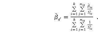
At L q, calculate the weighted least-squares estimate,
where n iq is the number of markers from study i that are within D cM of L q and where
The estimator for σ2 in equation (2), at L q, is
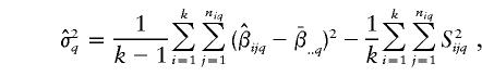
where is the average of
  that are within a window of D cM of L q, for _i_=1,…,k and _j_=1,…,n iq. The variance of
  is
is  .
. - 3.
Calculate the test statistic at L q : .
. - 4.
The analysis point L _q_′ that has the minimum, significant t q_′ value over the entire chromosomal segment is considered the most likely location (point estimate) of the gene locus. Thus, a point estimate of genetic variance, σ2_g, is .
.
Only the markers that are within a _D-cM window of L q are used in the estimate σ2_g, because of the positions of the markers relative to each analysis point. If a marker is linked (θ<0.50) to an analysis point, then the polymorphism at the marker can provide information about the polymorphism at the putative point.
Test for Homogeneity
To ensure that our meta-analysis test addresses the same linkage information, we propose the following test for homogeneity. At the analysis point L q_′,_ identified in step 4, where  , the homogeneity test statistic is
  , where
Under the assumption that σ2_q_=0, Q _q_′ follows an approximate χ2 distribution with  df (Gu et al. 1998). On the basis of the outcome of the homogeneity test, a linkage test is completed by comparing t _q_′ to an appropriate critical value from the standard normal distribution. In following section, we discuss several methods for the obtainment of such a critical value.
Simulations
We simulated a collection of five primary sib-pair linkage studies for a single QTL with no background polygenic variation and no shared sibling environment. We assumed random mating, Hardy-Weinberg equilibrium, and additive σ2_g_, within each study population. Five or 10 diallelic markers per study were uniformly positioned along a 100-cM chromosomal segment, such that no two studies could have markers at the same location. In particular, for the simulations with 5 markers per study, adjacent markers within the same study were 20 cM apart, and adjacent markers from different studies were 4 cM apart; likewise, for the simulations with 10 markers per study, adjacent markers within the same study were 10 cM apart, and adjacent markers from different studies were 2 cM apart. For simplicity, we assumed equal allele frequencies at all markers and at the QTL.
The genotypic data for the sib pairs were generated as follows:
- 1.
Parental-trait genotypes were simulated. - 2.
Parental-marker genotypes were simulated, under Hardy-Weinberg equilibrium, by use of allele frequencies and recombination fractions. - 3.
Sib-pair genotypes at each marker were generated from the appropriate parental marker gametes and recombination fractions.
Within each study j, the trait value for individual i, x ij, was simulated according to the model x _ij_=μ+g+ε, where μ is the overall phenotypic mean, g is the additive effect of a major diallelic gene, and ε is normally distributed error such that E(ε)=0, σ2ε=Var(ε), and Cov(g,ε)=0. We set μ=0, σ2_g_=1.0, and σ2ε=1.0, for all experiments. The heritability of the trait was set at 50%.
Within each study, both the proportion π of marker alleles shared IBD between sib pairs and the squared trait difference Y were calculated, for each sib pair, at each marker. The Haseman-Elston (1972) slope, at each marker, was determined by regression of Y on π. If homogeneity was refuted, then we did not conduct a linkage test. However, if homogeneity was not refuted, then we completed the meta-analysis (as described above, in the “Methods” section), with _D_=10 cM, to obtain estimates of location L _q_′ and genetic variance  . Experiments in which analysis points were placed 1.0 cM and 2.5 cM apart were completed. In all experiments, we simulated 1,000 replicates in five studies, with 1,000 sib pairs per study.
The Resampling SEs
Although the SE for  can be derived from the SE for
  (equation [1]), the SE for L _q_′ is not so readily attainable. Instead, we consider a resampling procedure, to obtain SE estimates for L _q_′. Using the same resampling procedure, we also obtained SEs for
  , to compare them to those derived from the meta-analysis procedure. The resampling procedure for the obtainment of SEs for L _q_′ and
  is as follows:
- 1.
Sample, with replacement, N data summaries from the pooled set of marker data summaries , where _N_=km , the total number of pooled markers available from all studies. For simulations with 5 markers per study, _N_=25, whereas, for simulations with 10 markers per study, _N_=50.
 - 2.
Complete the meta-analysis procedure (steps 1–4; see the “Methods” section), with the resampled set of markers. - 3.
At the analysis point where t _q_′_r_=min(t q r), retain the values for L q_′_r and , where r is the replicate index.
 - 4.
Repeat steps 1–3, for B replicates. - 5.
At the end of B replicates, calculate the resampling SEs for L _q_′ and as
as  and
and  , respectively.
Our reported SEs were obtained from _B_=500 resampling replicates.
Setting the Level of Significance
Linkage researchers debate how statistical significance should be determined in chromosomewide and genomewide scans. Two types of significance levels have been distinguished (Lander and Schork 1994): pointwise and genomewise. Chromosomewise significance levels may also be considered. The pointwise significance level is the probability that linkage would be identified at a given locus, when, in fact, the identified locus is not a QTL. The genomewise (chromosomewise) significance level is the probability that linkage would be identified somewhere in the entire genome (chromosome of interest) by chance alone.
Lander and Schork (1994) and Lander and Kruglyak (1995) discuss the importance and necessity, when multiple pointwise tests are being conducted throughout the genome, of controlling for a genomewise significance level in tests for linkage to complex-disease traits. Let α*T denote the desired genomewise false-positive rate, and let α_T_ denote the pointwise significance level that will be applied at each test point. Lander and Schork propose that an α*T appropriate to maintain the desired α_T_ be obtained by the relation

where C is the number of chromosomes in the genome, G is the genetic length (in Morgans) of the genome, and the constant ρ and the function h(T) are based on the crossing-over rate between the compared genotypes and on the distribution of the test statistic X, respectively. For sib pairs, ρ=2. When the test statistic is normally distributed, h(T)=_T_2. The T value in equation (3) is given by α*_T_=P(_X_>T), for the test statistic X. Lander and Schork assumed that a dense marker map was used in linkage analysis involving pedigree data and that the test statistic was either a LOD score or a normal score obtained from a test that was based on allele sharing among relatives.
Feingold et al. (1993) approximated significance levels by use of Gaussian-process models for genome scans that utilize affected-relative-pair data. The basis of their calculations is the approximation

where l is the length of the chromosome, β is twice the crossover rate per unit of genetic distance t, and Φ and φ are the functions of standard normal distribution and of density, respectively. Feingold et al. define Z t as a stationary Ornstein-Uhlenbeck process with mean 0 and covariance σ2_e_-β|t|, where σ2=p(1-p). For affected sib pairs, their critical value _b_=4.10 for β≈.05.
It has been argued (Sawcer et al. 1997, 1998; Kruglyak and Daly 1998) that these proposed pointwise P values may be excessively conservative, in testing for linkage within a single study. The appropriateness of these pointwise P values in meta-analysis has also been debated (Badner and Goldin 1999). In this application, we do not have a dense marker map, and a decision (i.e., hypothesis test) is made only for the analysis point that has the most extreme t q value. Failure to account for multiple testing may lead to an observed increase in false-positive results; however, a Bonferroni-type adjustment of the significance level may be too conservative for the meta-analytic procedure that we propose. For example, suppose that we use this meta-analytic procedure to combine Haseman-Elston results (for sib-pair analysis) across six studies that test for linkage in the same 100-cM region of a chromosome and that each study consider one analysis point every 2.5 cM, for a total of 41 analysis points. If the chromosomewise α level were set at 0.05, then the pointwise α level would be 0.05/41=0.001, which results in a pointwise critical value of −3.031. No adjustment to the α level would result in the well-known critical value of −1.645. By application of the method of Lander and Schork (1994) to this scenario, _C_=1, _G_=1, ρ=2, α*_T_=0.05, _T_=-1.645 (one sided), and h(T)=2.706; this calculation results in a pointwise significance value of α_T_=0.004 and in a pointwise critical value of −2.633. We conducted simulations under the null hypothesis of no linkage to the QTL, σ2_g_=0, with 1,000 replicates in five studies and with 1,000 sib pairs per study. We compared, at the meta-analytic level, the false-positive rates from the three previously discussed methods: unadjusted α level (NA), Bonferroni-adjusted α level (Bon), and the Lander and Schork (1994)–adjusted α level (LS). The NA critical value was −1.645; the Bon critical value was −3.031 for analysis points placed 2.5 cM apart; and the LS pointwise critical value was −2.633 (as stated above). We also considered equation (4), but the resultant critical value for our situation fell between the critical values obtained by Bon and LS methods. Hence, we included only Bon and LS critical values in our simulations. Because the underlying marker maps within each study were not dense, we opted for the conservative adjustment (i.e., Bon) of the significance level, for the linkage tests at the primary-study level. For _m_=5 markers per study, the pointwise significance level was  , with an associated critical value of −2.326; for _m_=10 markers per study, the pointwise significance level was
  , with an associated critical value of −2.576, from the standard normal distribution.
Simulation Results
Figure 1 presents the results of our simulation experiments for the QTLs positioned at 25 and 50 cM. The t q values were more extreme for analysis points that flank the putative QTL, and the location of the QTL was correctly identified. As expected, the location of the QTL was more pronounced (as indicated by smaller t q values) for simulations that contained 10 markers per study than it was for simulations that contained 5 markers per study. The meta-analysis estimates  at analysis points that flanked the QTL were similar for 5 and 10 markers per study; however, the SE of these estimates was considerably smaller (up to 60% smaller) when 10 markers per study were used. Although t q values were comparable in simulations with analysis points spaced every 1.0 and 2.5 cM, meta-analysis results of simulations with analysis points spaced every 2.5 cM were smoother in appearance. This finding could be a function of the window length, _D_=10 cM, that we used.
Figure 1.

Results (i.e., t q values), plotted for QTLs at 25 cM (a) and 50 cM (b), from meta-analyses with 5 markers per study and analysis points every 1.0 cM (large dots), 5 markers per study and analysis points every 2.5 cM (small, intermediate dots), 10 markers per study and analysis points every 1.0 cM (heavy, jagged line), and 10 markers per study and analysis points every 2.5 cM (light curve).
In all simulations, the most extreme test statistic occurred at the QTL; however, there was some variability. Figure 2 shows the distribution of the location of the most extreme t q values for simulations in which the QTL was at 50 cM. The variability was greater in simulations with five markers per study (fig. 2b and d). The distribution was clustered tighter around 50 cM in simulations with analysis points spaced every 1.0 cM (fig. 2c and d) as compared to analysis points spaced every 2.5 cM (fig. 2a and b). This tight clustering was a function of the space between analysis points, not of the meta-analytic procedure itself. Similar results (not shown) were observed when the QTL was at 25 cM.
Figure 2.

Distribution of the position (in cM) of the most extreme test statistic (i.e., t _q_′), plotted for a QTL at 50 cM, from meta-analyses with 10 markers per study and analysis points every 2.5 cM (a), 5 markers per study and analysis points every 2.5 cM (b), 10 markers per study and analysis points every 1.0 cM (c), and 5 markers per study and analysis points every 1.0 cM (d).
Table 1 shows the meta-analysis point estimates and the resampling-SE estimates for the location of the QTL and  . The resampling SEs were slightly smaller when analysis points were spaced every 1.0 cM than when they were spaced every 2.5 cM and, likewise, were smaller in simulations with 10 markers per study than in simulations with 5 markers per study. When D was increased to 20 cM, in the experiments with five markers per study, the resampling SEs were reduced, as was the bias in the estimates; for example, for the QTL at 25 cM, the estimate ± SE for location was 24.8±8.5 cM, and the estimate ± SE for σ2_g_ was 1.01±0.16. The
  SE that was derived from the meta-analysis procedure was comparable to that which had been obtained from resampling. For example, in the experiments with QTLs at 25 and 50 cM, with analysis points every 2.5 cM and with 10 markers per study, the meta-analysis
  was 0.14, and the resampling SE was 0.12 (table 1); in the simulations with analysis points spaced every 1.0 cM and with 10 markers per study, the meta-analysis
  was 0.13, and the resampling SE was 0.12 (table 1). Although the resampling and meta-analysis SEs for
  were comparable in the simulations with five markers per study, their were even more in agreement when _D_=20 cM than when _D_=10 cM.
Table 1.
Meta-analysis Point Estimates ± Resampling-SE Estimates of QTL Location and of σ2_g_ with Markers Uniformly Distributed Across a 100-cM Chromosomal Segment
| Mean Point Estimate ± Resampling-SEEstimate for Simulations with | ||||
|---|---|---|---|---|
| 5 Markers per Study,Analysis Points at | 10 Markers per Study,Analysis Points at | |||
| QTL | 1.0 cM | 2.5 cM | 1.0 cM | 2.5 cM |
| Location estimate: | ||||
| 25 cM | 25.0 ± 10.7 | 25.6 ± 11.2 | 25.0 ± 6.9 | 25.0 ± 7.3 |
| 50 cM | 50.2 ± 11.2 | 50.2 ± 11.4 | 50.2 ± 7.3 | 50.1 ± 7.5 |
| σ2_g_ Estimate: | ||||
| 25 cM | 1.02 ± .20 | 1.01 ± .20 | 1.01 ± .13 | 1.00 ± .14 |
| 50 cM | 1.02 ± .20 | 1.00 ± .20 | 1.00 ± .13 | 1.00 ± .14 |
The empirical power from the meta-analysis was >99% for all simulations in which empirical power at the primary-study level was low to moderate—ranging from 50.1% to 76.4%, at individual markers within 5 cM of the QTL—across all simulations. Table 2 contains the empirical type I error rates for both the meta-analytic procedure and the primary studies. The overall α level of 0.05 was maintained at the individual-study level by use of the Bonferroni adjustment. In the meta-analyses, the overall type I error rate varied not only with the type of adjustment proposed but also with the number of markers per study. No adjustment in the pointwise α level (i.e., NA) resulted in an inflated empirical α level as high as 41%! The LS method had type I errors that were slightly higher than the desired 5% level, for simulations with 10 markers per study, and type I errors that were slightly below the 5% level, for simulations with 5 markers per study. Bonferroni adjustment resulted in a conservative meta-analytic method, when either 5 or 10 markers per study were considered.
Table 2.
Empirical Type I Error Rates with Markers Uniformly Distributed Across a 100-cM Chromosomal Segment and Analysis Points Spaced Every 2.5 cM
| Empirical Type I Error Rates for Simulations with | ||||||||
|---|---|---|---|---|---|---|---|---|
| 5 Markers per Study | 10 Markers per Study | |||||||
| Meta-analysisa | Primary | Meta-analysisa | Primary | |||||
| QTL | NA | Bon | LS | Studyb | NA | Bon | LS | Studyb |
| 25 cM | 39.2 | 1.3 | 4.5 | 5.5 | 41.2 | 3.5 | 9.3 | 5.3 |
| 50 cM | 37.8 | 1.5 | 4.7 | 5.8 | 39.8 | 3.4 | 8.2 | 5.4 |
Adjustment of the α level by either method had no detrimental effect on the accuracy or precision of the estimates of either the location of the QTL or σ2_g_. The estimates of location differed by 10-2–10-3; the estimates for σ2_g_ differed by 10-4–10-5. The level of accuracy and precision would be expected to improve with an adjustment of the α level, since spurious linkages would occur less often. Clearly, some type of adjustment of pointwise α level is necessary when meta-analysis across a chromosome or genome is conducted. Further examination of the factors that need to be considered and included in such adjustment is warranted.
Between-Study Heterogeneity
Studies that test for linkage to the same QTL can differ in many ways, thereby leading to between-study heterogeneity. Types of heterogeneity include—but are not limited to—population heterogeneity (i.e., marker-allele frequencies varying across studies), marker heterogeneity (i.e., differing marker maps), ascertainment heterogeneity (i.e., differing ascertainment schemes), and environment heterogeneity (i.e., environmental exposures or effects varying across study populations). Studies may also differ on the basis of the amount of admixture in sample populations and on the basis of the definition of a phenotype (e.g., BMI and total or percentage body fat are two different measures of obesity).
In the previous set of experiments, the simulation parameters, except for the varying marker maps, were constant across all studies. Therefore, between-study variability was negligible. We conducted further experiments, to evaluate the meta-analytic method when between-study heterogeneity was not negligible. For these simulations, we considered 400 sib pairs per study. Within each study j, the trait value for individual i, x ij, was simulated as x ij_=μ+g j+e j+ε, where μ is the overall phenotypic mean, g j is the additive effect of the diallelic gene in study j, e j is the environmental effect in study j, and ε is the normally distributed error such that Cov(g j,e j)=Cov(e j,ε)=0 ∀_j . We set μ=0, σ2_g_ j_=1.0 ∀_j , and σ2ε=1.0 for all experiments but varied the amount of environmental variance (and, hence, heritability) across the studies, such that σ2_e_1=1.4, σ2_e_2=2.0, σ2_e_3=2.9, σ2_e_4=2.5, and σ2_e_5=1.8. We also simulated other marker maps for each study, such that the markers were not uniformly spaced. The chromosomal segment was divided into 5 or 10 equilengthed sections, and each study had, at most, one marker per section. Marker i in study j was randomly and distinctly located within section i of the 100-cM chromosomal segment, for all i and j, although one marker (namely, marker 1 in study 1) was at 0 cM and another marker (namely, the last marker in study 5) was at 100 cM. For simplicity, we assumed equal allele frequencies at all markers. The putative QTL was simulated at different positions along the chromosomal segment, for each simulation (25 and 50 cM). If homogeneity was refuted, then we did not conduct a linkage test. However, if homogeneity was not refuted, then we completed the meta-analysis (as described above, in the “Methods” section), in experiments with analysis points spaced every 2.5 cM. Figure 3 shows the two additional marker maps (which were combined for all studies) used in this set of simulation experiments.
Figure 3.

Position of randomly placed markers M ij, analysis points L q (only simulations with analysis points spaced every 2.5 cM are depicted), and gene loci (blackened circles), on the 100-cM chromosomal segment used in simulations. Each simulation experiment involved a single gene locus at each depicted location.
Heterogeneity-Simulation Results
Table 3 contains the results of the meta-analyses for three simulation sets:
- Series 1.
Markers were spaced uniformly, and σ2_e_=1.0 for all studies. - Series 2.
Markers were spaced uniformly, and σ2_e_ varied across studies (as stated above). - Series 3.
Marker maps were as depicted in figure 3, and σ2_e_ varied across studies, with the QTL at 25 cM.
Significant heterogeneity was detected in 10% of the experiments. We observed a slight increase in bias in point estimates and in resampling SEs of both location of the QTL and σ2_g_; this increase was due to the reduction of within-study sample size (series 1 compared to table 1). We again observed that the resampling SEs were slightly larger when only 5 (instead of 10) markers per study were simulated. Again, we increased D to 20 cM and observed a decrease in SEs and in bias of estimates, in the experiments with five markers per study. The resampling SEs were larger when the Lander and Schork (1994) adjustment was used instead of the Bonferroni adjustment: Recall that the Bon critical value (−3.031) was more extreme than the LS critical value (−2.633). The same increase in the resampling SEs for  were also observed for the SEs derived from the meta-analysis procedure. The point estimates for the location of the QTL were less biased when the Bon critical value was used; however, the point estimate for σ2_g_ was less biased when the LS critical value was used. Similar results were observed in simulations in which the QTL was at 50 cM (results not shown).
Table 3.
Meta-analysis Point Estimate ± Resampling SE of Location of QTL and σ2_g_ for a QTL at 25 cM, Analysis Points Every 2.5 cM, and Three Series[Note]
| Point Estimate ± Resampling SE for Simulations with | ||||
|---|---|---|---|---|
| 5 Markers per Study | 10 Markers per Study | |||
| Series | Bon | LS | Bon | LS |
| Location estimate: | ||||
| 1 | 26.4 ± 15.8 | 26.8 ± 16.9 | 25.4 ± 11.2 | 25.5 ± 11.8 |
| 2 | 26.4 ± 16.2 | 26.8 ± 17.0 | 25.1 ± 11.5 | 25.2 ± 11.9 |
| 3 | 26.3 ± 13.1 | 26.4 ± 14.6 | 25.2 ± 11.4 | 25.4 ± 12.1 |
| σ2_g_ Estimate: | ||||
| 1 | 1.13 ± .27 | 1.09 ± .28 | 1.03 ± .20 | 1.02 ± .20 |
| 2 | 1.12 ± .28 | 1.09 ± .30 | 1.01 ± .20 | 1.00 ± .20 |
| 3 | 1.12 ± .28 | 1.10 ± .29 | 1.05 ± .21 | 1.04 ± .22 |
Discussion
The meta-analytic method proposed herein is a simple tool for the consolidation of linkage information across several sib-pair studies. These simulations show that this method is useful in the detection of the major locus and does not require that the studies have a common marker map. This method simultaneously defines the location of the QTL and estimates genetic effect. In addition, this method permits a consensus test to be completed, after testing for homogeneity; and a final conclusion on the existence of linkage to a QTL can be made. SEs for the estimated location of the QTL can be obtained using a resampling procedure, and the user can choose to report SEs for  values derived by either the meta-analysis procedure or resampling.
Despite these advantages, the proposed method may be limited by other factors—including small-sample behavior (of the estimate of between-study variance and of the effect on homogeneity-test outcome and meta-analysis estimates), correlation of within-study marker information (and, in meta-analysis, the means to adjust for this correlation), an appropriate α-level adjustment, and the optimal value of D. We applied this meta-analytic method to the asthma data sets (i.e., genome scans) provided by Genetic Analysis Workshop 12 (Etzel and Costello 2001). We were not able, by this method (as described herein), to verify previously published linkage; however, no region definitively linked to asthma or a related trait has been consistently identified in the literature. The failure to verify such linkage may be due to the degree of population substructure and to the fact that the data were obtained from heterogeneous populations from around the globe. We completed simulations to investigate various types of between-study heterogeneity and their effects on meta-analyses (Etzel 2001). Variation among primary-study marker maps, population trait-allele frequencies, and environmental effects led to variation in the power to conclude linkage at the primary-study level. Power to conclude linkage at the pooled (i.e., meta-analytic) level was >90%, despite induced heterogeneity, and meta-analytic CIs for the location of the QTL and for genetic effect contained true parameter values at specified levels.
The meta-analytic method that we propose is used to detect one QTL, but we believe that meta-analysis will be useful in the detection of multiple QTLs that have not necessarily been localized to the same chromosome. Although we have presented this meta-analytic method by using the original Haseman-Elston (1972) procedure, any version of the Haseman-Elston method (e.g., see Elston et al. 2000; S. Shete, personal communication) could have been used in any of the primary studies. More generally, our approach is suitable for a collection of studies that use the same linkage statistic. One need only have individual statistics and their SEs, as well as the marker maps from each study. Thus, the method proposed herein could be applied to other situations (i.e., variance components), provided that the statistics used in the primary studies estimate the same population parameter.
Acknowledgments
We thank Christopher Amos, David Allison, and Tracy Costello for their generous support, helpful discussions, and comments on the manuscript. This work was supported, in part, by a cancer-prevention fellowship, National Cancer Institute grant R25 CA57730, and National Institutes of Health grants ES09912, HG02275, and R01 GM59506.
References
- Allison DB, Heo M (1998) Meta-analysis of linkage data under worst-case conditions: a demonstration using the human OB region. Genetics 148:859–865 [DOI] [PMC free article] [PubMed] [Google Scholar]
- Badner JA, Goldin LR (1999) Meta-analysis of linkage studies. Genet Epidemiol 17 Suppl 1:S485–S490 [DOI] [PubMed] [Google Scholar]
- Elston RC, Buxbaum S, Jacobs KB, Olson JM (2000) Haseman and Elston revisited. Genet Epidemiol 19:1–17 [DOI] [PubMed] [Google Scholar]
- Etzel CJ (2001) The impact of heterogeneity on meta-analysis of genetic linkage. Genet Epidemiol 21:151 [Google Scholar]
- Etzel CJ, Costello TJ (2001) Assessing linkage of immunoglobulin E using a meta-analysis approach. Genet Epidemiol 21 Suppl 1:S97–S102 [DOI] [PubMed] [Google Scholar]
- Feingold E, Brown PO, Siegmund D (1993) Gaussian-models for genetic linkage analysis using complete high-resolution maps of identity by descent. Am J Hum Genet 53:234–251 [PMC free article] [PubMed] [Google Scholar]
- Fisher RA (1925) Statistical methods for research workers, 13th ed. Oliver & Lloyd, New London, CT [Google Scholar]
- Folks JL (1984) Combination of independent tests. In: Krishnaiah PR, Sen PK (eds) Handbook of statistics 4. Elsevier Science, pp 113–121 [Google Scholar]
- Gu C, Province M, Todorov A, Rao DC (1998) Meta-analysis methodology for combining non-parametric sibpair linkage results: genetic homogeneity and identical markers. Genet Epidemiol 15:609–626 [DOI] [PubMed] [Google Scholar]
- Guerra R (2002) Meta-analysis in human genetic studies. In: Elston RC, Olson J, Palmer L (eds) Biostatistical genetics and genetic epidemiology. John Wiley & Sons, New York [Google Scholar]
- Guerra R, Etzel CJ, Goldstein DR, Sain SR (1999) Meta-analysis by combining p-values: simulated linkage studies. Genet Epidemiol 17 Suppl 1:S605–S609 [DOI] [PubMed] [Google Scholar]
- Haseman JK, Elston RC (1972) The investigation of linkage between a quantitative trait and marker locus. Behav Genet 2:3–19 [DOI] [PubMed] [Google Scholar]
- Hedges LV, Olkin I (1985) Statistical methods for meta-analysis. Academic Press, New York [Google Scholar]
- Kruglyak L, Daly MJ (1998) Linkage threshold for two-stage genome scans. Am J Hum Genet 62:994–996 [DOI] [PMC free article] [PubMed] [Google Scholar]
- Lander E, Kruglyak L (1995) Genetic dissection of complex traits: guidelines for interpreting and reporting linkage results. Nat Genet 11:241–247 [DOI] [PubMed] [Google Scholar]
- Lander ES, Schork NJ (1994) Genetic dissection of complex traits. Science 265:2037–2048 [DOI] [PubMed] [Google Scholar]
- Li Z, Rao DC (1996) Random effects model for meta-analysis of multiple quantitative sib pair linkage studies. Genetic Epidemiology 13:377–383 [DOI] [PubMed] [Google Scholar]
- Province MA (2001) The significance of not finding a gene. Am J Hum Genet 69:660–663 [DOI] [PMC free article] [PubMed] [Google Scholar]
- Rice JP (1997) The role of meta-analysis in linkage studies of complex traits. Am J Med Gen 74:112–114 [DOI] [PubMed] [Google Scholar]
- Risch N, Zhang H (1995) Extreme discordant sib pairs for mapping quantitative trait loci in humans. Science 268:1584–1589 [DOI] [PubMed] [Google Scholar]
- Sawcer S, Jones HB, Clayton D (1998) Response to Kruglyak. Am J Hum Genet 62:996–9979529366 [Google Scholar]
- Sawcer S, Jones HB, Judge D, Visser F, Compston A, Goodfellow PN, Clayton D (1997) Empirical genomewide significance levels established by whole genome simulations. Genet Epidemiol 14:223–229 [DOI] [PubMed] [Google Scholar]
- Wise LH, Lanchbury JS, Lewis CM (1999) Meta-analysis of genome scans. Ann Hum Genet 63:263–272 [DOI] [PubMed] [Google Scholar]