Population Snapshots Predict Early Hematopoietic and Erythroid Hierarchies (original) (raw)
. Author manuscript; available in PMC: 2018 Aug 21.
Published in final edited form as: Nature. 2018 Feb 21;555(7694):54–60. doi: 10.1038/nature25741
Abstract
Red cell formation begins with the differentiation of multipotent hematopoietic progenitors. Reconstructing the steps of differentiation represents a stereotypical challenge in stem cell biology. Combining single-cell transcriptomics, fate assays, and theory for predicting fate from population snapshots, we inferred a continuous, hierarchical structure of murine hematopoietic progenitors committing to seven blood lineages. We uncovered coupling between erythroid and basophil/mast cell fates, a global hematopoietic response to erythroid stress, and novel growth factor receptor regulators of erythropoiesis. We also defined a new flow-cytometric sorting strategy to purify progressive early stages of erythroid differentiation, completely isolating classically-defined burst-forming (BFU-e) and colony-forming progenitors (CFU-e). Intriguingly, profound remodeling of the cell cycle is intimately entwined with erythroid development and with a sharp transcriptional switch that extinguishes the CFU-e stage and activates terminal differentiation. Our work showcases the utility of theory linking transcriptomic data to predictive fate models, providing insights into lineage development in vivo.
Introduction
The abundance of erythroid progenitors in hematopoietic tissue provides a unique opportunity for dissecting how multipotent progenitors (MPPs) differentiate into a single lineage in situ, a process of fundamental biological interest and of clinical relevance. Erythropoiesis has two principal phases: erythroid terminal differentiation (ETD), where Gata1-driven transcription remodels erythroid precursors into red cells through several well-described stages1–3; and an earlier, less well delineated phase of early erythropoiesis, where the hematopoietic stem cell (HSC), through poorly defined intermediates, gives rise to erythroid progenitors, identified by their colony-forming potential in semi-solid medium, as BFU-e and CFU-e4,5. A direct, complete and high-purity isolation of adult murine BFU-e and CFU-e from hematopoietic tissue has not been attained6–9. More broadly, there have been no strategies that systematically identify the entire cellular and molecular trajectory of the early erythroid lineage as it first arises from the HSC and progresses to the point where ETD is activated.
Probing the earliest stages of erythropoiesis requires exploring how MPPs diversify into progenitors for each of the hematopoietic lineages. Single cell approaches have recently upended established models of hematopoiesis, showing that progenitor populations that were thought to be similar in their developmental stage and fate potentials are in fact highly heterogeneous in both respects10–17. Alternative models replaced the classic hematopoietic tree18–20 with a ‘flatter’ hierarchy, in which uni-lineage progenitors derive directly from a heterogeneous set of lineage-biased multipotent progenitors. These new models are highly dependent on the tools employed in the analysis of high-dimensional cell transcriptional states, which are currently undergoing intense innovation21–26. Descriptions of the hematopoietic structure have so far relied on clustering12, which may fail to capture continuum behaviors; diffusion maps26,27, which are powerful for branching models but provide less detail of highly complex processes; and the ordering of progenitors based on their similarity to differentiated cell types16, which may overlook progenitors that do not resemble mature cells. Fluorescence-activated cell sorting (FACS) may also introduce bias into reconstructed developmental trajectories, through restrictive gates15 and loss of sensitive cells28. It is still not clear how to reconcile cell fate assays with cell state maps proposed from single cell profiling, and indeed this remains a general challenge in stem cell biology.
Here we investigated the derivation and subsequent development of erythroid progenitors by undertaking single-cell RNA-seq (scRNA-seq) of a broad set of hematopoietic progenitors, using the inDrops platform29. We developed an analytical tool, Population Balance Analysis (PBA), that predicts fate probabilities from static snapshots of single cell transcriptomes through dynamic inference, which allowed us to define a FACS strategy to isolate cells in progressive stages of early erythropoiesis. Using single cell fate assays, we then confirmed a number of detailed predictions regarding the early hematopoietic hierarchy and erythroid developmental progression. The insights obtained regarding early erythropoietic fate control may be applicable to other differentiation models, and include novel erythropoietic regulators with potential translational relevance.
Results
Single-cell RNA-seq of Kit+ progenitors
We performed scRNA-Seq on Kit+ hematopoietic progenitor cells (HPCs) isolated using magnetic beads from murine adult bone marrow (BM) (Fig. 1a). Kit is expressed on all hematopoietic stem and early progenitor cells30,31, allowing an inclusive approach that preserves the relative abundance of progenitor cell states. After filtering, we carried forward 4,763 HPC transcriptomes for analysis (see Data Availability for interactive tools).
Figure 1. The early hematopoietic hierarchy predicted by scRNA-seq.
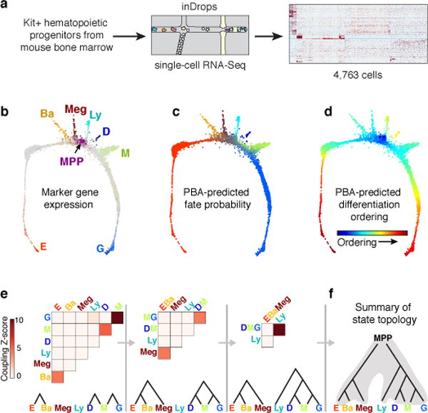
a Schematic for scRNA-seq of Kit+ mouse bone marrow.
b SPRING plots of single-cell transcriptomes. Each point is one cell. Colors indicate lineage-specific gene expression. E, erythroid; Ba, basophilic; Meg, megakaryocytic; Ly, lymphocytic; D, dendritic; M, monocytic; G, neutrophil granulocytes; MPP, multipotential progenitors.
c,d Parameterization of the cell state graph using PBA, encoding the graph position of each cell by a set of predicted fate probabilities (c) (colors as in (b)), and pseudo-temporal ordering with MPPs at the origin, terminating with the most mature observed cells of each lineage (d).
e,f A cell state hierarchy encodes the cell graph topology. Lineage-biased states were identified by comparing the fraction of cells with PBA-predicted bilineage coupling with expected values from fate randomization (e). Iteratively joining fates based on pairwise coupling revealed the cell state hierarchy (f).
We visualized the scRNA-Seq data using the SPRING algorithm32 (Fig. 1b), which generates a graph of cells (graph nodes) connected to their nearest neighbors in gene expression space, projected into two dimensions using a force-directed graph layout. This visualization suggested that HPCs occupy a continuum of transcriptional states, rather than discrete metastable states, a result which contrasts with single cell data from mature blood lineages and is supported by formal tests of graph interconnectivity (Extended Data Fig. 1a). When SPRING plots were colored based on expression of lineage-specific markers (Fig. 1b, Supplementary Table 1), the cells were found to organize around an undifferentiated core, from which seven distinct branches emerge, corresponding to progenitors of granulocytic neutrophils (G), monocytic (M), dendritic (D), lymphoid (Ly), megakaryocytic (Meg), basophilic/mast cell (Ba), and erythroid (E) lineages. Although this structure depends critically on collecting cells using a broad selection marker, SPRING visualization of data from previous studies12,15 revealed the same lineage relationships (Extended Data Fig. 1b).
Population Balance Analysis of the HPC continuum
To understand the differentiation trajectories that cells might follow, we developed Population Balance Analysis (PBA)33, an approach for studying single cell continua (Extended Data Fig. 1c–d). PBA maps each cell to a low-dimensional space that encodes the cell graph topology in the form of predicted cell fate probabilities. The derivation and limitations of PBA are detailed elsewhere33. The core of PBA can be understood as reconstructing a memoryless stochastic dynamics of cells, which, through ongoing cell turnover, explains the observed steady-state distribution of cell states. PBA approximates the dynamics of cells as following the gradient of a potential landscape, which itself can be inferred through an asymptotic relationship between diffusion-drift processes and the spectral properties of the SPRING graph33. The probabilities obtained by PBA represent formal biophysical predictions for the fate of cells under simplified assumptions, but they can also be treated heuristically as encoding graph distances. Applied to our data, for each hematopoietic progenitor, PBA defines seven putative commitment probabilities (Fig. 1c, Extended Data Fig. 1e), as well as the distance from the undifferentiated CD34hi/Sca1hi MPPs (Fig. 1d).
The transcriptional state continuum of HPCs is hierarchical, but not a strict tree
We used PBA-predicted commitment probabilities to compute a coupling score that reflects whether any two fate potentials co-occur in the same progenitor, at rates higher than expected by chance (Fig. 1e). A transcriptional state hierarchy was formalized by identifying correlated pairs of terminal fates, joined iteratively until a multipotent state was reached (Fig. 1e,f).
The resulting topology firmly supports the hierarchical view of hematopoiesis, with MPPs diverging into progenitors with correlated E/Meg/Ba fates, or correlated Ly/Myeloid fates (Fig. 1f). However, the transcriptional-state hierarchy emerges from correlations on a continuum, rather than from discrete populations. Additionally, it predicts two refinements over current models: first, the erythroid fate is correlated with the basophil/mast cell fates. Second, among myeloid progenitors we identified dendritic-monocyte (DM) and granulocytic-monocyte (GM) coupling, but no DG coupling, suggesting that monocyte differentiation may occur through two distinct trajectories, a prediction that was very recently independently confirmed34. The PBA-formalized HPC hierarchy also allowed us to identify genes whose expression closely correlates with each cell fate choice (Extended Data Fig. 2, Supplementary Table 2).
scRNA-Seq-guided isolation of putative erythroid progenitors
To test PBA predictions (Fig. 1e–f), we developed a flow cytometric strategy which isolates scRNA-Seq-defined hematopoietic subpopulations. Guided by the single cell expression patterns, we combined Kit expression with CD55, a marker of Meg/E bias10; Kit+CD55+ cells were subdivided into P1 to P5, using CD49f (Itga6) and Meg/E markers6,10,9 (Fig. 2a). Using qRT-PCR (Extended Data Fig. 3a), and scRNA-Seq (11,241 cells post-filter) (Fig. 2b, Extended Data Fig. 3b–e), we mapped cells from each of the sorted subpopulations back to regions of the SPRING graph. We found that P1 and P2 represent high-purity subpopulations on the putative erythroid branch, with P1 predicted to be committed, and P2 mostly committed, to the erythroid fate (Fig. 1c). P3 and P4 are enriched for the basophilic and megakaryocytic branches, respectively; P3 further bifurcates into basophil and mast cell branches. P5 contains erythroid-biased oligopotent and multipotent cells. Myeloid, lymphoid and some MPP states are within the CD55− zone of the plot.
Figure 2. A novel sorting scheme isolates erythroid progenitors.
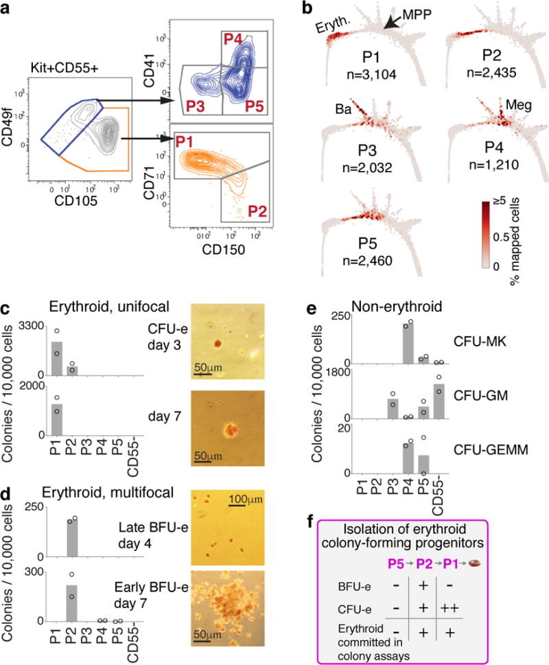
a Kit+CD55+ BM cells were sorted into gates P1 to P5, and profiled using scRNA-Seq.
b P1-P5 single cell transcriptomes localized to their most similar counterparts on the SPRING graph.
c-e Colony formation by P1-P5 and Kit+CD55− cells. Bars are mean of n=2 independent experiments (circles), each performed in triplicate. Images show erythroid colonies, stained for hemoglobin with diaminobenzidine. Colonies: CFU-MK=Megakaryocytic (Extended Data Fig. 4a), CFU-GM= granulocytic/monocytic; CFU-GEMM= mixed myeloid.
f Summary of erythroid colony potential of FACS subsets.
Fate assays identify correlated cell fates and early E/Ba/Meg progenitors
We next examined the differentiation potential of the sorted P1-P5 populations, and by extension, the predicted fate probabilities for their corresponding transcriptional states. Colony forming assays showed that P1 and P2 contain all of the unipotential erythroid progenitors and no other progenitors (Fig. 2c–e). P1 colonies were small and unifocal (Fig. 2c), maturing on day 3 (CFU-e) or later, whereas P2 colonies were largely multifocal, maturing on day 4 or later (BFU-e) (Fig. 2d). Thus, P1 is closer to erythroid maturation than P2, consistent with PBA predictions (Fig. 2b, Fig. 1c). Further, the molecular stage of progenitors determines their ability to form either multifocal or unifocal colonies. In agreement with the SPRING plot, the less differentiated P5 gave rise to mixed myeloid colonies, and P4 was enriched for CFU-Mk (Fig. 2e, Extended Data Fig. 4a).
To further test HPC fate potential, we sorted single Kit+ cells into liquid culture wells in the presence of cytokines supporting myeloid and erythroid differentiation (Fig. 3a). We assayed the clonal output of 1,158 single cells by FACS (Fig. 3b, Extended Data Fig. 4b). Unipotential clones for the E, Ba, Meg and G/M lineages largely originated in the P1/P2, P3, P4 and CD55− subpopulations, respectively, consistent with predictions (Figs 3b, 1c, 2b). Many clones contained multiple lineages, with strong, statistically significant couplings between the E, Ba and Meg cell fates on the one hand, and the G and M fates on the other (Fig. 3c; z-score absolute value > 10 compared to randomized data), consistent with both known (E/Meg, G/M) and novel (E/Ba) PBA predictions (Fig. 1c, e–f). Progenitors with E/Ba output were enriched in P2 and P5 (Fig. 3d), which map close to the E/Ba branch point in the scRNA-Seq data (Figs. 2b, 1c), and were depleted in the CD55− population, also as predicted. We found similar results in bulk liquid cultures (Extended Data Fig. 4c). Of note, the new basophil differentiation pathway suggested by our data does not rule out basophil formation by the traditional route, as some clones gave rise to G/Ba fates. These results suggest that E/Ba/Meg fates are coupled transcriptionally and functionally, while being anti-coupled to the G/M fates, and that scRNA-Seq data can be used to generate successful predictions of HPC states and fates.
Figure 3. Predicted fate couplings confirmed by single cell fate assays.
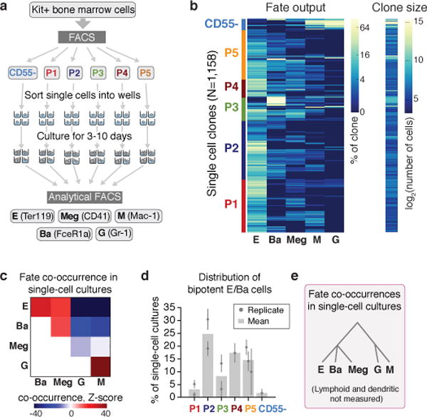
a Schematic of single cell liquid cultures, measuring clonal output with the indicated antibodies.
b Lineage output (left) and size (right) of each clone (rows) as in (a).
c Lineage co-occurrences in (b), computed by comparing the number of clones producing a pair of fates to the number expected following randomization.
d Fraction of bipotent erythroid-basophil (EBa) clones in P1-P5, containing E and Ba cells, but no other fates. Individual points and error bars show the expectation value and standard error from independent single cell sorting experiments. Bars represent the mean of n=two (P1, P2, P3) or n=three (P5) independent experiments; a single experiment was performed for P4 and CD55-.
e Cell state hierarchy based on fate co-occurrence in single-cell cultures.
The erythroid differentiation trajectory
Integrating the cell fate assays and scRNA-Seq analysis, we partitioned the continuum of cell states between MPPs and ETD into three stages (Fig. 4a): (1) erythroid-basophil-megakaryocytic progenitors (EBMegP), (2) early erythroid progenitors (EEP), and (3) committed erythroid progenitors (CEP). EBMegPs are oligopotent cells near branch points to megakaryocytic and basophil lineages, biased away from the G/M fates, and strongly represented in P5 and P2 (Fig. 2b). EEPs occupy a narrow region of the graph, just past the final non-erythroid fate branch point, form most of P2, and are functionally BFU-e (Fig. 2b–d). CEPs constitute the majority of unipotential erythroid progenitors, form most of P1, and are functionally CFU-e (Fig. 2b–d).
Figure 4. Stages of early erythropoiesis and the global erythroid stress response.
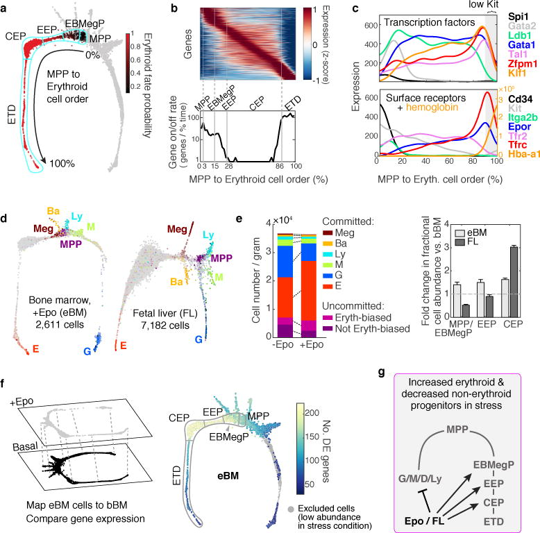
a Erythroid trajectory stages between MPP and erythroid terminal differentiation (ETD): EBMegP, Erythroid-Basophil-Megakaryocyte biased progenitors; EEP, Early Erythroid Progenitors; CEP, Committed Erythroid Progenitors. The SPRING plot shows PBA-predicted erythroid fate probability.
b Top: dynamically varying genes (rows), ordered by peak expression, in cells (columns) ordered from MPP to ETD. Gene expression smoothed using a Gaussian kernel. Bottom: number of genes turning on or off (density of expression inflection points) with progression from MPP to ETD. The x-axis represents PBA-predicted differentiation ordering of cell transcriptomes, uniformly spaced from the least (0%) to the most differentiated (100%).
c Gene expression traces for established erythroid genes.
d SPRING plots of eBM and FL. Cells colored as in Fig. 1b.
e Left: Erythroid lineage expansion at the expense of non-erythroid cells (see Extended Data Fig. 7). Among uncommitted cells, erythroid-biased progenitors increased, while the remainder diminished. Committed cells were defined by a PBA-predicted erythroid fate probability >0.5. Right: relative change in each progenitor stage relative to basal bone marrow. Error bars are the sampling standard error (n=1 sample per condition).
f Epo stimulated differential gene expression. Cells from eBM were first mapped onto the basal BM SPRING plot, followed by analysis of differentially-expressed (DE) genes.
g Summary of the stress erythropoiesis response.
To establish the transcriptional events of the erythroid trajectory, we created a smoothed time series for every gene from MPP to ETD, akin to published pseudotemporal ordering algorithms35,36,37 (Fig. 4b). Known erythroid regulators recapitulated expected expression dynamics (Fig. 4c). Gata1 and the erythropoietin (Epo) receptor, EpoR, were induced early, concurrent with suppression of Spi1 (PU.1) and _Gata_238. The transition to ETD was marked by sharp induction of erythroid genes such as α-globin (Hba-a1). We validated expression of canonical transcription factors in sorted P1-P5, including the early expression of Gata1 (Extended Data Fig. 5a,b). We further established that a graded increase in Tfrc (CD71) is a reliable marker of continuous progression through the EEP and CEP stages, finding that transcriptomes of sorted CD71high P1 cells map to late CEP stage, and that CD71 gradually increases in sorted P2 and P1 cells differentiating in vitro (Extended Data Fig. 5c–d). A further, sharp increase in CD71/Tfrc takes place at the transition to ETD (Fig. 4c).
Of ~4,500 genes that varied significantly along the erythroid trajectory (Supplementary Table 3), a large group was induced at the onset of the CEP stage, and sharply suppressed at the CEP/ETD transition (Fig. 4b). It contained the most dominant dynamic gene clusters, enriched for cell cycle and growth-related genes, including mTOR signaling, nucleotide metabolism, and DNA replication (Extended Data Figs. 5e, 6a,b and Supplementary Table 4). These pathways suggest that the CEPs, which are the most abundant cells in early erythropoiesis, act as an “amplification” module. Our analysis predicts new erythroid epigenetic and transcriptional regulators (Extended Data Fig. 6 and Supplementary Table 4), and interestingly, shows that while Gata1 is expressed early in the erythroid trajectory, the majority of its canonical targets are induced only at the transition to ETD. Taken together, the temporal ordering of the single-cell transcriptomes recapitulates known events of early erythropoiesis and uncovers a dedicated CEP transcriptional program that is distinct from the ETD program.
Stress generates erythroid-trajectory-wide changes but preserves the hematopoietic topology
We examined two models of accelerated, or stress, erythropoiesis, using scRNA-Seq: the mid-gestation fetal liver (FL; _N_=7,182 cells post-filter), where erythropoiesis is rate limiting to fetal growth, and bone marrow from mice treated with Epo for 48 hours, stimulating red cell production (eBM; _N_=2,611 cells post-filter). SPRING graphs revealed a remarkable conservation of the key features of the hematopoietic hierarchy and erythroid differentiation during stress (Fig. 4d). The proportion of erythroid trajectory cells increased with stress (Figs 4d,e). In FL, the increase was predominantly in CEPs, whereas, surprisingly, in eBM, all erythroid trajectory cells increased in abundance, including uncommitted MPPs and EBMegPs. This increase was at the expense of other lineages, since the absolute number of Kit+ cells in eBM did not change (Fig. 4e and Extended Data Fig. 7). A number of mechanisms could account for this, including altered intrinsic fate bias of MPPs39,40.
Epo altered gene expression principally in EEPs and CEPs, but also in EBMegPs and MPPs (Fig. 4f), including downregulated targets of C/EBPβ, a transcription factor that biases differentiation away from erythroid/megakaryocytic fates41. We identified both known42,43 and new stress-responsive genes, together with their precise localization within the erythroid trajectory (Extended Data Fig. 8, Supplementary Table 5).
Taken together, we found that the cell state branching structure is maintained during accelerated erythropoiesis. We identified changes in gene expression and in cell abundance in response to Epo, in MPPs and throughout the ensuing erythroid progression, well beyond the currently known mechanism of Epo-driven erythropoietic expansion44,42.
Novel growth factor regulators of early erythropoiesis
We screened EEP and CEP for expression of cell-surface receptors with known ligands, identifying three such receptors: Ryk, Mst1r and Il17ra (Fig. 5a, Extended Data 9a, b). Ryk and Mst1r were previously found in CFU-e, but their functions remained unknown45,46. However, the expression of an IL-17 receptor by early erythroid progenitors had not been documented. We stimulated Ryk, Mst1r and IL-17Ra with their respective ligands, Wnt5a, MSP and IL-17a, using erythroid colony formation as readout (Fig. 5b, Extended Data Fig. 9c). In FL in the presence of low Epo (50 mU/ml), MSP doubled the number of CFU-e colonies, equivalent to a 10-fold increase in Epo concentration. MSP was inhibitory in other contexts, and Wnt5a was a potent inhibitor of all erythroid colony formation in both FL and BM. By contrast, IL-17a mediated a striking potentiation of adult BM CFU-e colony formation, quadrupling colonies at lower Epo (50mU/ml), and increasing them by ~50% in high Epo.
Figure 5. Novel growth factor regulators of early erythropoiesis.
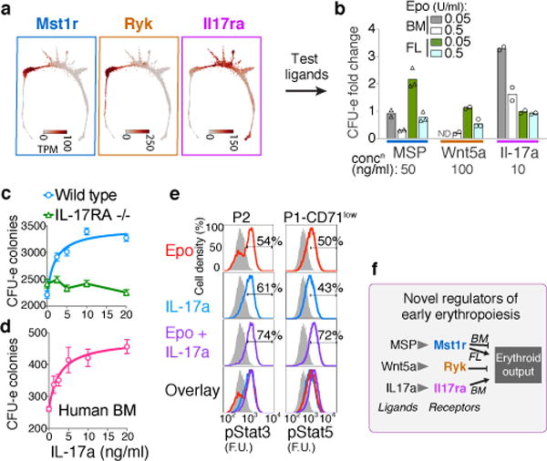
a Expression patterns for Mst1r, Ryk and Il17ra. See Extended Data Fig. 9a,b.
b Effect of MSP, Wnt5a or Il17a on Epo-dependent CFU-e colony formation. Bars are means of n=2 or 3 independent experiments (individual data points), each performed in quadruplicate. Full analysis in Extended Data Fig. 9c.
c The IL-17a response is lost in IL-17Ra−/− BM. Mean ± SD per 500,000 BM cells plated in triplicate in the presence of Epo (0.05 U/ml); representative of two independent experiments.
d IL-17a stimulates CFU-e formation in freshly isolated human BM mononuclear cells. Mean ± SD per 85,000 cells plated in triplicates.
e IL-17a –mediated phosphorylation of Stat3 and Stat5 (pStat3, pStat5). Fresh BM cells were starved of cytokines for 3 hours, and then stimulated with either Epo, IL-17a or both; FACS profiles are for baseline (starved, in grey), and 60 minutes –post stimulation (in color). Representative of 2 independent experiments, each performed in duplicate.
f Summary of novel growth factor effects on erythroid output.
The stimulatory effect of IL-17a required endogenous IL-17Ra (Fig 5c) and was also evident in human BM (Fig 5d). Further, IL-17a stimulation was saturable, with a low EC50 (60 pM), consistent with high affinity-binding of IL-17a to IL-17Ra. IL-17a induced rapid phosphorylation of the intracellular signaling mediators Stat3 and Stat5 in CEP and EEP (Fig. 5e), and freshly sorted CEP/P1 and EEP/P2 expressed IL-17Ra by western blotting (Extended Data Fig. 9d). Taken together, our findings suggest previously unknown regulation of EEP and CEP through the expression of a number of growth factor receptors new to erythropoiesis.
Extensive remodeling of the cell cycle during erythroid developmental progression
In a final analysis, we asked what governs progression through the CEP stage and its termination at the ETD. We previously reported that ETD onset in the FL occurs within a single S phase, and is dependent on S phase progression47; further, this unique S phase is shorter and faster than S phase in pre-ETD cells48,49. These conclusions, based on analysis of large FL subpopulations, predict that CEP exit should show an S phase signature. In our scRNA-Seq data, we found that genes whose expression marks G1/S, S, G2 and G2/M cell cycle phases indeed form a sequence of close, sharp peaks during CEP exit, likely representing a single cell cycle (Fig. 6a–b). This and the following results hold even when cell cycle genes are omitted for ordering the erythroid trajectory (Extended Data Fig. 10a–c). Significantly, by reversibly inhibiting DNA replication, we found that the CEP/ETD transition in adult BM not only synchronized with, but also depended on, S phase progression (Extended Data Fig. 10d–f).
Figure 6. Extensive remodeling of the cell cycle during erythroid development.
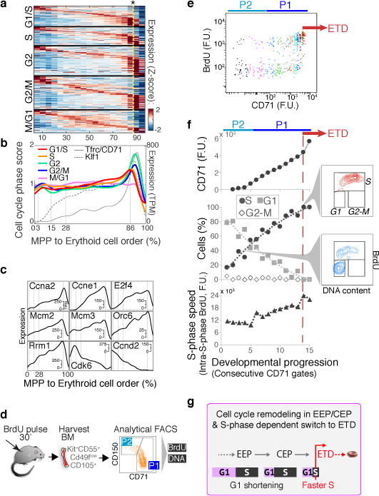
a Cell-cycle-phase specific genes52, ordered by peak expression, reveal cell-cycle synchronization with the CEP/ETD transition (indicated by *).
b Mean expression of all genes specific to each cell cycle phase (as in (a)), traced along the erythroid trajectory. ETD is activated with a sharp Tfrc/CD71 upregulation.
c Representative cell cycle genes correlated or anti-correlated with erythroid trajectory progression.
d Schematic for cell cycle analysis of erythroid progenitors in vivo. BM was harvested and fixed 30 min following BrdU injection; P1 and P2 cells were analyzed for BrdU incorporation and DNA content.
e BrdU-labeled S phase cells, as in (d). Cell coloring represents consecutive 7-percentile gates of increasing CD71, reflecting progression through P2/EEP and P1/CEP (Extended Data Fig. 5c,d). Transition to ETD (red arrow) is marked by a sharp CD71 increase, and synchronization in S phase (BrdU+).
f CD71 expression (top), cell cycle phase distribution (middle), and intra-S phase DNA synthesis rate (lower panel), for all gates in ‘e’. Insets show representative cell cycle distribution FACS plots. Representative of three independent experiments. Similar eBM and FL analysis is in Extended Data Fig. 10g.
g Summary of cell cycle remodeling during early erythropoiesis.
The scRNA-seq data revealed that changes to cell cycle machinery occur throughout CEP, perhaps in preparation for the switch to ETD. Genes whose expression most closely correlates with CEP progression (Supplementary Table 6) are enriched for Gene Ontology terms associated with DNA replication. Strikingly, regulators of S phase and the G1/S transition increase steadily through the CEP stage, including Cyclin E1 (Ccne1), Cyclin A2 (Ccna2), and Mcm helicase subunits (Mcm2-7). Conversely, the G1 phase regulators, Cyclin D2 (Ccnd2) and Cdk6, decrease steadily (Fig. 6c). To investigate these findings, we labeled S phase cells in vivo with the nucleotide analog BrdU, and analyzed the cell cycle distribution of cells as they progressed through the EEP/CEP stages (Fig. 6d–f). We found a graded but dramatic increase in the fraction of cells in S phase, while the number of G1 cells correspondingly decreased. Similar results held in eBM and in FL (Extended Data Fig. 10g). There was no significant change in S phase speed/length, evidenced by stable intra-S phase BrdU48 (Fig. 6f); suggesting that cells spend more time in S phase as a result of G1 shortening. Western blotting of sorted P1 and P2 fractions confirmed the increasing expression of key S phase regulators with developmental progression in EEP/CEP (Extended Data Fig. 10h). Taken together, our data suggest that progression through the erythroid trajectory is associated with extensive remodeling of the cell cycle (Fig. 6g).
Discussion
Our scRNA-seq analysis reveals that HPCs occupy a continuum of transcriptional cell states, branching towards 7 fates. Certain cell fate potentials are correlated, supporting a hierarchical view of hematopoiesis, with MPPs diverging either towards myeloid and lymphoid fates, or towards the erythroid/megakaryocyte/basophil cell fates. Yet unlike the classical models of hematopoiesis, HPCs do not separate into discrete and homogenous stages. The coupling of specific cell fates, which we validated with single-cell fate assays, is a critical feature by which our model differs from recent models of hematopoiesis, where uni-lineage progenitors arise directly from MPPs. Our model also explains historical hierarchical interpretations of hematopoiesis, which were based on fate assays of FACS-gated populations, averaging the fate couplings of their constituent progenitors. Of note, the continuum nature of the scRNA-Seq data does not rule out the existence of discrete epigenetic or signaling states among HPCs, if their lifetime in single cells is comparable to, or shorter than, the lifetime of mRNA molecules (hours to ~1 day).
We delineated the continuous differentiation trajectory of the erythroid lineage, from its origins in MPPs, through EBMegPs, to unipotential EEPs and CEPs, which we show correspond to the unipotential BFU-e and CFU-e, respectively. The dominant CEP stage expresses a distinct transcriptional program, and is a likely regulator of erythroid output, as evidenced by its expansion in stress, and by novel growth factor receptors that regulate CEP/CFU-e number. These include strong stimulation by the pro-inflammatory IL-17Ra, possibly contributing to the growing evidence of complex interplay between erythropoiesis and inflammation50,51. We further identified the cell cycle as a key process in both the progression and termination of the CEP stage. Developing CEPs spend an increasing fraction of their time in S phase, as a result of G1 shortening; their transition to ETD in an abrupt transcriptional switch is dependent on a single, short S phase. We speculate that the cell cycle may set the context for activation of transcription factors which are induced earlier in the erythroid trajectory. Taken together, our single cell approach allowed us to make detailed predictions which we validated to reveal novel fundamentals of early hematopoietic differentiation, as well as practical methods for further isolation and study of these cells.
METHODS
Single-cell RNA-seq
Mice
For the basal state bone marrow sample (bBM), and for the sorted populations P1 to P5, bone marrow was harvested from 8-week old adult BALB/cJ female mice (Jackson Laboratories, Maine, USA). For the Epo-stimulated adult bone-marrow sample (eBM), 8-week old adult Balb/cJ female mice were injected with Epo (Procrit, Amgen corporation) sub-cutaneously once per 24 hours for a total of 48 hours, at 100 Units/25 g. For the fetal liver sample (FL), BALB/cJ female mice were set up for timed pregnancies, and fetal livers were harvested on embryonic day 13.5.
Cell preparation
Tissue harvesting
For bone-marrow preparation, femurs and tibiae were harvested immediately following euthanasia, and placed in cold (4°C) ‘staining buffer’ (phosphate-buffered saline (PBS) containing 0.2% Bovine Serum Albumin (BSA) and 0.08% Glucose). Bones were flushed using a 2 mL syringe with a 26-gauge needle and then crushed with a pestle and mortar to obtain all cells. Harvested bone marrow cells were filtered through a 40 μm strainer and washed in cold ‘Easy Sep’ buffer (PBS; 2% fetal bovine serum (FBS); 1mM EDTA). Fetal livers were prepared by mechanical dissociation in staining buffer and a wash in ‘Easy-Sep’ buffer.
Positive selection for Kit+ cells
Bone marrow and fetal liver cell samples were each enriched for Kit expressing cells using magnetic beads, with the Mouse Biotin Selection Kit (STEMCELL technologies [Cat # 18556]) and Biotin Rat Anti-Mouse CD117 antibody (clone 2B8, BD Bioscience), following the manufacturer’s protocol.
Density gradient centrifugation
Following magnetic bead selection, dead cells and debris were removed from the bone marrow and fetal liver samples using density centrifugation in OptiPrep (Sigma, Cat # D1556). Briefly, cells were re-suspended in 0.5ml staining buffer, mixed with 1mL of 40% of Optiprep in PBS, and placed in a 5 mL tube. The cell suspension was carefully over-layered with 2 mL of 20% OptiPrep solution, and 1mL of 5% OptiPrep solution, and centrifuged at 800g for 15 min (Centrifuge break OFF). The top visible cell band that formed during centrifugation contained the live, Kit+ single cells, confirmed by flow cytometric analysis. This layer was carefully aspirated and used directly in the inDrops29 platform.
Single cell transcriptome droplet microfluidic barcoding using inDrops
For scRNA-seq, we used inDrops29 following the protocol previously described53 with the modifications summarized in Supplementary Table 7. Following droplet barcoding reverse transcription, emulsions were split into aliquots of approximately 1000 single cell transcriptomes and frozen at −80C. Two batches of Kit+ libraries were prepared, referred to as Batch 1 (bBM, n=840 cells; eBM, n=1,141 cells; FL, n=1,953 cells) and Batch 2 (bBM, n=4,592 cells; eBM, n=1,314 cells; FL, n=7,529 cells) in Supplementary Table 7. These cell numbers correspond to the final number of transcriptomes detected upon sequencing (see “Cell filtering and normalization” below), and were in agreement with estimated inputs.
For the FACS subsets P1, P1-CD71hi, P2, P3, P4, and P5 (referred to collectively as “P1-P5”), all libraries were prepared in parallel, with a total of 16,206 cell barcodes detected in the sequencing data prior to filtering (P1, n=5,733 cells; P1-CD71hi, n=1,631 cells; P2, n=2,630 cells; P3, n=2,101 cells; P4, n=1,589 cells; P5, n=2,522 cells).
Sequencing and read mapping
The first batch of Kit+ (bBM, eBM, FL) libraries was sequenced on a HiSeq 2000, the remaining Kit+ libraries were sequenced on three NextSeq 500 runs, and all P1-P5 libraries were sequenced on a single NextSeq 500 run. Raw sequencing data (FASTQ files) were processed using the inDrops.py bioinformatics pipeline available at github.com/indrops/indrops and described in53, with a few modifications. Bowtie version 1.1.1 was used with parameter –e 100; all ambiguously mapped reads were excluded from analysis; and reads were aligned to the Ensemble release 81 mouse mm10 cDNA reference.
Cell filtering and data normalization
Each sample (bBM, eBM, FL, P1-P5) was processed separately. The bBM, eBM, and FL samples (referred to collectively as “Kit+”) were initially filtered to include only abundant barcodes, based on visual inspection of the histograms of total reads per cell (see cell numbers reported in “Single cell transcriptome droplet microfluidic barcoding using inDrops”). An additional filtering step removed cells with transcript count totals in the bottom 5th percentile (bBM, n=271 cells; eBM, n=148; FL, n=473). Subsets P1-P5 were filtered only by total transcript counts, with thresholds set by visual inspection of the total counts histograms (see cell numbers reported in “Single cell transcriptome droplet microfluidic barcoding using inDrops”). Next, we excluded putatively stressed or dying cells with >10% (bBM, eBM, FL) or >20% (P1-P5) of their transcripts coming from mitochondrial genes (bBM, n=165 cells; eBM, n=45; FL, n=698; P1, n=2,629; P1-CD71hi, n=879; P2, n=195; P3, n=69; P4, n=379; P5, n=62).
After cell filtering, we detected the following median number of transcripts and genes per cell, respectively: bBM: 2,989 and 1,539; eBM: 3,082 and 1,552; FL: 8,859 and 2,834; P8: 3,339 and 1,637; P8-CD71hi: 4,740 and 2,174; P9: 2,712 and 1,393; P10: 4,641 and 2,158; P11: 1,783 and 1,023; P12: 2,139 and 1,195.
Each cell’s gene expression counts were then normalized using a variant of total-count normalization that avoids distortion from very highly expressed genes. Specifically, we calculated x^i,j, the normalized transcript counts for gene j in cell i, from the raw counts xi,j as follows: x^i,j=xi,jX¯/Xi, where Xi= ∑jxi,j and X¯ is the average of Xi over all cells. To prevent very highly expressed genes (e.g., hemoglobin) from correspondingly decreasing the relative expression of other genes, we excluded genes comprising >10% of any cell’s total counts when calculating X¯ and Xi.
Exclusion of contaminating cell types and putative cell doublets
To clean up the data for the Kit+ samples, we clustered the single cell transcriptomes and excluded clusters that were identified as contaminating (non-HPC) cell types and putative cell doublets. No such clusters were detected in the P1-P5 samples. Clustering was performed as follows: we identified principal variable genes across the entire data set, as described in29 i.e. genes that were highly variable (top 2000 most variable by v-score, a measure of above-Poisson noise [variability]), were expressed at non-negligible levels (at least 5 UMI-filtered mapped reads [UMIFM] in at least 3 cells), and which contributed to principal components with eigenvalues above those obtained following data randomization (n=59, n=35, n=71 principal components for bBM, eBM and FL samples, respectively). The expression level for each gene was standardized by a z-score transform (mean-subtraction, scaling by standard deviation), followed by density-based clustering (DBSCAN)54,55 on a 2D PCA-tSNE plot (principal component analysis [PCA] followed by t-distributed stochastic neighbor embedding [tSNE56] as described in29,57). The tSNE algorithm perplexity parameter was set to 30. Examination of marker gene expression in each cluster was then used to identify putative doublets and contaminating cell types.
In the bBM sample, two doublet clusters were identified: one co-expressed markers of mature macrophages and erythrocytes (n=38 cells), while the other co-expressed markers of granulocyte and erythroid progenitors (n=75 cells). The eBM sample included a cluster of mature macrophages (n=40 cells) but no identifiable cluster of doublets. The FL sample contained four contaminating cell types: vascular endothelium, hepatocytes, mesenchymal cells, and mature macrophages (n=769 cells total), in addition to a small cluster of doublets (n=18 cells). Doublets and contaminant cells were excluded from downstream analyses.
To increase confidence that putative doublet clusters were indeed combinations of two single cells, rather than true intermediate/transitional states, we generated simulated “artificial” doublets by randomly sampling and combining observed transcriptomes.
We then applied PCA-tSNE clustering as described above to the union of observed and simulated cells, and identified clusters that were primarily composed of cells with a large number of doublet neighbors (two clusters in bBM, one in FL). These clusters were the same putative doublet clusters identified in the previous paragraph.
Batch correction
Within each Kit+ sample, we observed batch effects between the first and second sequencing runs, with slightly fewer genes detected per cell in the second run compared to the first run. This was consistent with the choice of lower sequencing depth used in the second set of runs, but could also reflect differences in library preparation despite all cells being collected in a single droplet run. To prevent batch effects from distorting subsequent data analysis, for each sample we used the second (larger) batch to select variable genes and to calculate principal component (PC) gene loadings. Cells from all batches were then projected into the reduced space, and all subsequent analysis was performed on the reduced PC space.
Data visualization and construction of k-nearest neighbor (KNN) graphs
Following cell filtering, data was prepared for visualization and Population Balance Analysis (PBA)33 by constructing a kNN graph, in which cells correspond to graph nodes and edges connect cells to their nearest neighbors. A kNN graph was constructed separately for each of the three Kit+ samples and for the merged P1-P5 samples (note that the kNN graph for P1-P5 was used only for the visualization in Extended Data Fig. 3).
For the Kit+ samples, genes with mean expression >0.05 and coefficient of variation (standard deviation/mean) >2 were used to perform principal components analysis (PCA) down to 60 dimensions (bBM, eBM, FL). For all analyses in this paper, data were z-score normalized at the gene level prior to PCA (qualitatively similar results were also obtained without z-score normalization, which weights highly expressed genes more heavily than lowly expressed genes). After PCA, a kNN graph (k=5) was constructed by connecting each cell to its five nearest neighbors (using Euclidean distance in the PC space).
For P1-P5, highly variable genes were filtered using the v-score statistic (above-Poisson noise) rather than CV, keeping the top 25% most highly variable genes and requiring least 3 UMIFM detected in at least 3 cells (n=3,459 genes). Additionally, a strong cell cycle signature was observed in the initial graph visualization, manifested by co-localization of cells expressing G2/M genes (Ube2c, Hmgb2, Hmgn2, Tuba1b, Mki67, Ccnb1, Tubb, Top2a, Tubb4b). Therefore, we constructed a G2/M signature score by summing the average z-score of these genes, then removed genes highly correlated (Pearson r > 0.2) with the signature (n=31 genes). Finally, the kNN graph was constructed with k=4 using the first 30 PCs.
The kNN graphs were visualized using a force-directed layout using a custom interactive software interface called SPRING58. For the Kit+ samples, several manual steps were taken to improve visualization. It is important to emphasize that the manipulations affect visualization only. All subsequent analyses depend on the graph adjacency matrix, which is not affected by any of the changes to the graph layout. For visualization purposes, we manually extended the length of the Mk, Ba, and Mo branches by pinning the position of cells at the end of each branch, and allowing the remaining structure to follow. In the bBM sample, we compressed the CEP “bulge” region of the graph by bringing its bounding cells together.
Smoothing over the kNN graph
We smoothed data over the kNN graph for gene expression visualization and for one analysis (“Global changes in gene expression in stress conditions”). Smoothing was done by diffusing the property of interest (e.g., gene expression counts or number of mapped cells) over the graph, as described in59. In brief, let A be the adjacency matrix of the kNN graph, where _Ai,j_=1 if an edge in the graph connects nodes i and j. Define A* as the transition matrix, obtained by row-normalizing A:
Let Ei be the quantity of interest (e.g., expression level) in cell i. Then E*, the smoothed vector of E, is computed as follows:
where γ is a diffusion constant (γ=0.05 in all presented analyses) and I is the identity matrix.
Formal measure of the continuity of transcriptional states
To demonstrate that the continuum appearance of the Kit+ transcriptomes was not a trivial outcome of our analysis methods, we used the same tools to analyze an scRNA-seq dataset of mature blood cells (peripheral blood mononuclear cells, PBMCs) [https://support.10xgenomics.com/single-cell-gene-expression/datasets/2.0.1/pbmc8k], which consist of several distinct cell types (Extended Data Fig. 1a). In addition to generating a SPRING plot of the data, we also assessed each dataset’s interconnectivity by examining the behavior of random walks over the kNN graphs, as in Velten et al.16. In detail, after subsampling the PBMC data to contain the same number of cells as the bBM dataset, we applied PCA and constructed a kNN graph (k=10) for each dataset. We then simulated 1,000 random walks for each graph and plotted the fraction of nodes (cells) visited as a function of the number of steps (Extended Data Fig. 1a).
Population balance analysis (PBA)
The PBA algorithm calculates for each cell a scalar “potential” that is analogous to a distance, or pseudotime, from an undifferentiated source, and a vector of fate probabilities that indicate the distance to fate branch points. These fate probabilities and temporal ordering were computed using the python implementation of PBA (available online https://github.com/AllonKleinLab/PBA), as described in Weinreb et al.33.
The inputs to the PBA scripts are a set of csv files encoding: the edge list of a k-nearest neighbor graph of the cell transcriptomes (A.csv); a vector assigning a net source/sink rate to each graph node (R.csv); and a lineage-specific binary matrix identifying the subset of graph nodes that reside at the tips of branches (S.csv). These files are provided in the Supplementary Data for the BM and FL data sets. PBA is then run according to the following steps:
- Apply the script “compute_Linv.py –e A.csv”, here inputting edges (flag “–e”) from the SPRING kNN graph (see previous Methods section). This step outputs the random-walk graph Laplacian, Linv.npy.
- Apply the script “compute_potential.py –L Linv.npy –R R.csv”, here inputting the inverse graph Laplacian (flag “-L”) computed in step (1) and the net source/sink rate to each graph node (flag “-R”). This step yields a potential vector, V.npy, that is used for temporal ordering (cells ordered from high to low potential). The vector R provided in the Supplementary Data was estimated as described in the next section.
- Apply the script “compute_fate_probabilities.py –S S.csv –V V.npy –e A.csv –D 1”, here inputting the lineage-specific exit rate matrix (flag “-S”), the potential (flag “-V”) computed in step (2), the same edges (flag “-e”) used in step (1) and a diffusion constant (flat “-D”) 1. This step yields fate probabilities for each cell.
Front end Figures 1–6 make use of PBA analyses of bBM data. For Fig. 4e and Extended Data Fig. 8, a temporal ordering of erythroid differentiation was generated for the FL data set using the same steps, with input files also provided in Supplementary Data.
Estimation of net source/sink rate vector R
Theory
A complete definition of the vector R in terms of biophysical quantities is provided in Weinreb et al.33. In brief, for a gene expression space described by a vector _x_=(_x_1,_x_2,…,_x_N) giving the expression of each of N genes, R(x) gives the net imbalance between cell division and cell loss locally for cells with gene expression profile x. R(x) is corrected for cell enrichment and loss resulting from experimental procedures such as sample enrichment, as follows. In this experiment, all progenitors including HSCs express Kit, but eventually down-regulate it as they terminally differentiate. Thus, no cells enter the experimental system other than through proliferation of existing Kit+ HPCs, but the selection for _Kit_+ cells during sample isolation induces a net sink on cells down-regulating Kit expression. For a self-renewing system, cell division and cell loss are precisely balanced, so ∫R(x)dx=0. To apply PBA, one does not need to estimate R(x), but only its value at points xi at which the M cells _i_=1,…,M are observed in the scRNA-Seq measurement. Thus R is a vector over the cells in the system. For a self-renewing system, the sum over all cells satisfies the same constraint, ∑iRi=0.
Estimation of R
We assigned negative values to R for the top 10 cells with highest marker gene expression for each of the seven terminal lineages (see Supplementary Table 1 for marker genes), which were separately confirmed to show reduced Kit expression. We assigned different exit rates to each of the seven lineages using a fitting procedure that ensured that cells identified as putative HSCs would have a uniform probability to become each fate. Putative HSCs were identified by the similarity of their transcriptomes to microarray profiles from the ImmGen database (we used SC.LT34F.BM [long-term BM HSCs] for bBM and SC.STSL.FL [short-term FL HSCs] for FL; for more details, see section “ImmGen Bayesian classifier” below). We assigned a single positive value to all remaining cells, with the value chosen to enforce the steady-state condition ∑iRi=0. In the fitting procedure, all exit rates are initially set to 1 and iteratively incremented or decremented until the average fate probabilities of the putative HSCs were within 1% of uniform. The resulting vector R is provided in the Supplementary Data file. The separate lineage exit rates were then used to form the lineage-specific exit rate matrix S, provided in the Supplementary Data.
Assignment of PBA fate probabilities and temporal ordering to eBM dataset
We assigned to each of the eBM cells the average temporal order (or potential V) and average fate probabilities of the 20 mostly similar basal BM cells. To do this, we first carried out a principal component analysis (PCA) on the basal BM cells into 60 dimensions. We then used the gene loadings of the 60 PCs to project the eBM data into the same PC space. The distance of each eBM cell to each basal BM neighbors was then measured by cosine distance in the 60-dimensional sub-space.
ImmGen Bayesian classifier
We used a published microarray profile60 to search for similar cells in our own dataset using a naïve Bayesian classifier, implemented as follows.
The Bayesian classifier assigns cells to microarray profiles based on the Likelihood of each microarray profile for each cell, with the Likelihood calculated by assuming that individual mRNA molecules in each cell are multinomially sampled with the probability of each gene proportional to the microarray expression value for that gene. Consider a matrix E of mRNA counts (UMIs) with n rows (for cells) and g columns (for genes), and also a matrix M with m rows (for microarray profiles) and g columns for genes. M was quantile normalized and then each microarray profile was normalized to sum to one. E was normalized as in section “Cell filtering and data normalization”. The (n×m) matrix Sij giving the Likelihood of each microarray profile j for each cell i is,
where Zi is a normalization constant that ensures ∑iSij=1.
Computing the hematopoietic lineage tree
We used the fate probabilities from PBA to infer the topology of the hematopoietic lineage tree using an iterative approach (Fig. 1e–f). Each iteration began with a set of fates and a probability distribution over those fates for each cell. For every pair of fates, we computed a fate coupling score (see next paragraph) and merged pairs with a score significantly higher than expected under a null model. The merged fates inherited probabilities from the starting fates by simple pairwise addition.
The coupling score between two fates A and B is the number of cells with P(A)P(B) > ε, where we used a value ε=1/14 throughout. To generate a null distribution for each fate pair, we computed pairwise coupling scores for 1000 permutations of the original fate probabilities. The heatmaps in Fig. 1e show z-scores with respect to these null distributions.
Analysis of fate-correlated genes at hematopoietic choice-points
To discover fate-associated genes at key choice points in hematopoiesis (Extended Data Fig. 2; Supplementary Table 2), we ranked transcription factors (TFs) and cell surface markers (TFs from http://genome.gsc.riken.jp/TFdb/tf_list.html, surface markers from http://www.ebioscience.com/resources/mouse-cd-chart.htm) by their correlation with PBA-predicted fate probability, restricting to cells that were bi-potent for the given choice. Specifically, to find TFs associated with fate A at an A/B choice point, we first selected cells with P(A)∗P(B) > ε, (ε=1/14) and then ranked the TFs by their correlation with the fate bias [P(A)−P(B)]. In Supplementary Table 2, we report all genes with Pearson significance p < 0.01 (Bonferroni corrected). In Extended Data Fig. 2, we show at most 10 genes for any one choice point.
Mapping P1-P5 subsets to the Kit+ graphs
For Fig. 2b, cells from subsets P1-P5 were projected into the same PC space as the bBM data, then mapped to their most similar Kit+ neighbors. In detail, first, counts were converted to transcripts per million (TPM) for all samples. Then, using only the bBM cells, the 3000 most highly variable genes (measured by v-score) with at least 3 UMIFM in at 3 cells were z-score normalized and used to find the top 50 principal components. Next, the P1-P5 subset cells were z-score normalized using the gene means and standard deviations from the bBM data and transformed into the bBM PC space. Lastly, each P1-P5 cell was mapped to it closest bBM neighbor in PC space (Euclidean distance).
Extracting MPP-to-Erythroid trajectory cells
To isolate the erythroid trajectory, we defined an MPP-to-erythroid axis in each of the three Kit+ datasets by ordering cells based on their graph distance from unbiased MPPs (cells identified based on the ImmGen classifier as described above), and keeping only cells for which the probability of erythroid fate increased or remained constant with graph distance. Graph distance was measured by PBA potential, and starting with the cell closest to the HSC origin, we added the cell with next-highest potential to the trajectory if the PBA-predicted erythroid probability for cell i was at least 95% of the average erythroid probability of the cell(s) already in the trajectory.
More formally the procedure is as follows: order all N cells in the experiment from highest to lowest PBA potential V, with decreasing potential corresponding to increasing distance from MPPs33. Let Ei be an indicator variable for the membership of ordered cell i in the erythroid trajectory (Ei = 1 if cell i is in the trajectory; otherwise, Ei = 0). If Pi is the PBA-predicted erythroid probability for ordered cell i, then Ei=1 if
Erythroid trajectory cells were then ordered by decreasing potential. Defining tj as the index of the jth erythroid trajectory cell,
Throughout the paper, we report this cell order (akin to the “pseudotime” reported in other publications) as a percent of ordered cells, with the first, least differentiated cell at 0% and the most mature cell at 100%. This is not meant to suggest that erythroid differentiation ends with this final observed cell.
Identifying dynamically varying genes
For each gene, a sliding window (n=100 cells) across the MPP-to-Erythroid ordering was used to identify the windows with maximum and minimum average expression as in57. At-test was then performed to assess the statistical significance of the difference in expression levels. To estimate the false-discovery rate (FDR), we permuted the order of the cells and repeated the above analysis57. For a p-value generated by the observed (non-permuted) ordering, the FDR-corrected p-value is the fraction of genes from the permuted ordering with that p-value or less. Any gene with an FDR-corrected p-value <0.05 was considered significantly variable.
Identifying stage transitions in MPP-to-Erythroid trajectory
Transition points between stages of erythropoiesis were defined using the frequency of gene inflection points (Fig. 4b), patterns of PBA-predicted fate probabilities (Fig. 1c), and the fate potentials of FACS subsets P1-P5 (Figs. 2,3). That said, due to the continuous nature of the transcriptional states, the locations of these transitions should be considered approximate.
The inflection point density is the number of genes turning on or off at a given point on the trajectory. For each gene, inflection points were identified as the points with maximally increasing or decreasing expression as follows: first, each dynamically varying gene’s trajectory was smoothed using Gaussian smoothing with a width σ=5% of total trajectory. The gene expression derivative for gene k, denoted xk', was then computed by taking a 10-cell moving average of the difference between consecutive smoothed gene expression values. Inflection points were then identified as the points with maximum or minimum derivative for each gene. To exclude maxima or minima resulting from relatively small gene expression fluctuations, only appreciably large extrema were kept for further analysis. Specifically, the point with the maximum derivative for gene k, max(xk'), was kept only if
max(xk')median(abs(xk'))>Q.
Minima were similarly filtered, requiring the ratio to be <-Q. We chose a threshold _Q_=6, but results do not qualitatively change over a range of Q. We then plotted the density of these inflection points over the MPP-to-erythroid axis. Regions with large-scale gene expression changes have a high density of inflection points, while a low density characterizes relatively stable states.
Dynamic gene clustering
Dynamically varying genes were clustered based on their behavior at the transition points. To prevent overfitting, we used only three transitions (3%, 18%, 86%) by splitting the EEP state and assigning the first and second halves to the EBMP and CEP states respectively. At each transition, genes were classified as increasing, decreasing, or unchanging, giving a total of 33=27 possible patterns. After smoothing gene expression traces, the data were binned by calculating the mean expression in each of the four stages. To remove noisy genes or genes that varied little across bins, we calculated the range of binned expression values, range(xi,binned)=max(xi,binned)−min(xi,binned), for each gene and proceeded with the top 50% most variable genes. Next, to place all genes on a similar scale, each gene’s binned expression values were divided by its maximum binned value. Finally, the differences between consecutive bins were thresholded: differences > 0.15 were called increasing, differences < −0.15 were called decreasing, and differences >−0.15, <0.15 were called unchanging.
Gene set enrichment analysis (GSEA)
Each of the 27 gene clusters was used as input for GSEA (Hypergeometric test), using all genes as background. Ribosomal genes were excluded from the input, as were predicted genes (Gm*). Gene sets from MSigDB v5.161 from the following list were tested for enrichment: Hallmark (h.all.v5.1.symbols.gmt), C2 curated canonical pathways (c2.cp.v5.1.symbols.gmt), C3 transcription factor targets (c3.tft.v5.1.symbols.gmt), and C5 Gene Ontology (c5.all.v5.1.symbols.gmt). Additionally, for transcription factor target (TFT) enrichment analysis, we used gene sets from the ChEA database62.
Cell cycle phase analysis
Genes with periodic expression correlated with the cell cycle in HeLa cells52 were used to generate a cell cycle phase score for each cell. The list of phase-specific genes was filtered to exclude genes with a mean expression >25 TPM in MPP-to-erythroid trajectory cells. For Fig. 6a, a sliding window average was computed using a window size of 10% MPP-to-erythroid progression (~200 cells) and a jump size of 5%. For Fig. 6b, counts were normalized by the mean expression at the gene level, and smoothed using Gaussian smoothing. Then, for each phase (G1/S, S, G2/M, M, M/G1), a phase score was calculated by averaging the smoothed gene expression traces for the genes specific to that phase.
Testing the influence of cell cycle genes on MPP to Erythroid cell order
To test the extent to which cell cycle genes influenced the ordering of cells along the MPP to Erythroid trajectory, we excluded annotated cell cycle genes (as in63) – a combination of genes from the Gene Ontology database (GO:0007049) and Cyclebase64 – and repeated kNN graph construction and PBA. As shown in Extended Data Fig. 10, the resulting cell order was largely unchanged, as were the dynamics of cell cycle genes.
Identifying genes that change steadily in the CEP stage
To identify genes that are steadily up- or down-regulated throughout the CEP (Fig. 6c and Supplementary Table 6), we tested each gene’s magnitude of change (slope) and the linearity of its change (the error of the actual gene trace from a straight line). Restricting to cells in the CEP stage and genes with at least 2 UMIFM in at least 5 cells, we fit a linear regression to the ordered gene expression values and also generated a smoothed expression trace using a Gaussian kernel (width σ=5%). We then computed a “linearity score” for each gene by dividing the slope of the regression line by the root-mean-square error between the regression line and smoothed trace. Steadily increasing genes receive large positive scores, while steadily decreasing genes are assigned a large negative score. Genes that do not change much or that change non-linearly (e.g., sharply increasing only at the end of the stage) receive scores close to 0.
Global changes in gene expression in stress conditions
Cells from eBM and FL (stress samples) were mapped to their most similar bBM counterparts, and differentially expressed genes were identified. Mapping was carried out by applying PCA to the bBM and stress samples and finding the closest 20 bBM neighbors for each stress cell. Specifically, the input genes were the principal variable genes described in the “Cell filtering and data normalization” section. Counts matrices were z-score normalized separately for each sample, and PCA was performed on the basal sample to obtain the gene loadings. Using the top 60 PCs, each sample was then transformed using these coefficients, thereby projecting the cells into the same PCA space. To validate this mapping method, we performed the same procedure using different subsets of bBM data as training and test sets (see “Validation of cross-sample cell mapping” below)
Each stress cell’s 20 closest bBM neighbors (Euclidean distance) were found, and for the purpose of comparing gene expression, each of these k (20) neighbors inherited 1/k (1/20) of the transcript counts from the mapped stress cell. To enable the comparison of regions of gene expression space (as opposed to comparing single mapped cells to single basal cells), the mapped and original gene expression values were smoothed over the kNN graph, as described in a previous section (“Smoothing over the kNN graph”). To avoid comparing gene expression patterns in regions that were relatively unpopulated in the stress sample (e.g., parts of the granulocyte branch), we smoothed the number of mapped stress cells per basal cell over the graph and then excluded basal cells with few mapped stress cells (number mapped cells <=9 for eBM and <=20 for FL).
A differential expression score for each cell i and gene j was defined as the max-normalized difference between mapped and basal expression, x^i,j∗ and x^i,j, respectively:
di,j=x^i,j∗−x^i,j0.5⋅(max(x^j∗)+max(x^j))
A gene level score, Dj, was created by summing over the cells, Dj=∑idi, j. Genes were considered differentially expressed if
Dj>D¯+2⋅σD or Dj<D¯−2⋅σD,
where D¯ is the average over all gene level scores Dj and σD is the standard deviation.
Then, for each differentially expressed gene, the gene was counted as differentially expressed at a given cell if
di,j>0.5⋅δhigh or di,j<0.5⋅δlow,
where δhigh is the 99th percentile of Dj and δlow is the 1st percentile of Dj.
Validation of cross-sample cell mapping
To test the accuracy of the method for mapping eBM and FL cells to bBM cells, we divided the bBM sample into a test training set (random sample of 75% of the cells) and training test set (the remaining 25%). The mapping procedure described in the previous section was then used to map the test set to the training set. As one measure of the accuracy of the mapping, we assigned the test cells the average PBA-predicted fate probabilities and differentiation ordering of the training cells to which they mapped. Both measures were relatively unchanged from their original values (Spearman correlation of 0.97 for the differentiation ordering and >0.95 for each fate probability). As a second measure, we repeated the test for finding global changes in gene expression, using the same gene level score (Dj) cutoff as for the eBM. This revealed no significantly differentially expressed genes between the training and test sets.
Region-specific differential expression
Prior to identifying differentially expressed genes, we excluded genes with large batch effects. While different sequencing depths led to a small change in the average expression of many genes from the first batch to the second, a small number of genes showed major batch effects beyond this, presumably due to differences in library prep. We performed a binomial test for differential expression65 between the two batches of cells and excluded genes with p<10−50, resulting in the removal of 461 genes.
In general, genes can be differentially expressed globally or only in specific cell populations. Particularly when comparing FL to bBM, many genes showed global up- or down-regulation. In order to identify differentially expressed genes likely to important specifically for erythropoiesis (or in a particular stage of erythropoiesis), we created a region-specific differential expression score, described in detail below. This score measures the magnitude of the expression difference within a region of interest (ROI) relative to the magnitude outside the region; genes with a larger difference within the ROI than outside of it receive a high score (positive for up-regulation, negative for down-regulation). For the analyses in this paper, we tested for differential expression in five ROIs: the erythroid trajectory stages EBMP, EEP, CEP, and ETD, plus an expanded selection of “MPP” cells, which included cells with a maximum PBA-predicted lineage probability (for all lineages) <0.4, excepting cells already included in one of the erythroid trajectory stages.
After mapping stress cells to their single closest neighbor in bBM (as described in the previous section), we selected bBM cells in the ROI and the stress cells mapping to them. We first identified genes differentially expressed within the ROI by performing a binomial test for differential expression65, which tests the probability that a gene is expressed more frequently in one population than another. After correcting for multiple hypothesis testing (Benjamini-Hochberg procedure66), we proceeded with genes with an FDR-corrected p-value <0.05.
To identify genes differentially expressed specifically within the ROI and not elsewhere, we calculated the mean-normalized expression difference for ROI cells and non-ROI cells for the significant binomial test genes. For two samples, A (stress) and B (basal), the mean-normalized expression difference of gene i within the ROI, yin,i, is
yin,i=x¯in,iA−x¯in,iB(x¯all,iA+x¯all,iB)/2 ,
where x¯in,iA is the average expression of gene i within the ROI in sample A. A similar score was calculated for cells outside the ROI:
yout,i=x¯out,iA−x¯out,iB(x¯all,iA+x¯all,iB)/2
Plotting yin,i vs. yout,i clearly reveals genes more highly DE within the ROI than without. A single score per gene was computed as follows:
scorei={max(yin,i−max(yout,i,0),0), if yin,i>0min(yin,i−min(yout,i,0),0), if yin,i<0
Intuitively, this score is large and positive if a gene is more strongly upregulated within the ROI than without, is large and negative if a gene is more strongly downregulated within the ROI than without, and is close to 0 otherwise.
To build gene lists for GSEA input, we first selected genes with scorei>0.1∗max(score) (for upregulated genes) or scorei<0.1∗min(score) (for downregulated genes) and then used the top 100 genes by binomial test p-value.
Flow cytometric sorting for P1 to P5 subsets
A detailed protocol of this procedure was submitted to protocol exhange67.
Bone marrow cells from adult BALB/cJ male or female mice, ages 8-12 weeks, were lineage-depleted using the Mouse Streptavidin RapidSpheres Isolation Kit (STEMCELL Technologies [Cat# 19860A]), with the following biotinylated antibodies:
- anti-CD11b (Clone M1/70 [#557395], BD Biosciences)
- anti-Ly-6G and Ly-6C (Clone RB6-8C5 [#553125], BD Biosciences)
- anti-CD4 (Clone RM4-5 [#553045], BD Biosciences)
- anti-CD8a (Ly-2) (Clone 53-6.7 [#553029], BD Bioscience)
- anti-CD19 (Clone 1D3 [#553784], BD Biosciences)
- anti-TER119 (Clone TER119 [#553672], BD Biosciences).
Lineage-depleted cells were then labeled with the following antibodies in the presence of 1% rat serum:
- streptavidin Alexa Fluor 488 (Molecular Probes), to mark lineage-positive cells
- CD117-APC Cy7 (Clone 2B8 [#105826], Biolegend)
- TER119-BUV395 (Clone TER-119 [#563827], BD Biosciences)
- CD71-PE Cy7 (Clone RI7217 [#113812], Biolegend)
- CD55-AF647 (Clone RIKO-3 [#131806], Biolegend)
- CD105-PE (Clone MJ7/18 [#120408], Biolegend)
- CD150-BV650 (Clone TC15-12F12.2 [#115931], Biolgened)
- CD41-BV605 (Clone MWReg30 [#133921], Biolegend)
- CD49f (=itga6) – BV421 (Clone GoH3 [#313624], Biolegend)
Following washes, cells were re-suspended in DAPI-containing buffer and sorting was performed on BD FACSAria II with a 100 μ nozzle. Sorted populations were defined as in Fig. 2a.
qRT-PCR on sorted populations
RNA was prepared from sorted cell subsets using the RNeasy Micro Kit (QIAGEN; CAT# 74004) or TRIzol reagent (Ambion; CAT# 15596026), and measured with RiboGreen RNA reagent kit (Thermo Scientific) on the 3300 NanoDrop Fluorospectrometer. cDNA was synthesized using the same amount of input RNA for all samples in a parallel reaction, using the Super Script III first-strand synthesis system for RT-PCR (Invitrogen) with random hexamer primers. The ABI 7300 sequence detection system, TaqMan reagents and TagMan MGB probes (Applied Biosystems, San Diego, CA) were used following the manufacturer’s instructions. qPCR was carried on 4 serial dilutions of each cDNA sample, and the linear part of the template dilution/signal response curve was used to calculate relative mRNA concentrations following normalization to β-actin, using the ΔCt method.
The following TagMan MGB probes were used:
Mst1r (Mm00436382_m1), Ryk (Mm01238551_m1), IL17ra (Mm00434214_m1), Mt2 (Mm00809556_s1), Slc26a1 (Mm01198850_m1), Slc4a1 (Mm00441492_m1), Trib2 (Mm00454876_m1), Cd34 (Mm00519283_m1), Meis1 (Mm00487664_m1), Hpn (Mm01152654_m1), Pf4 (Mm00451315_g1), Dntt, (Mm00493500_m1), Ms4a2 (Mm00442778_m1), Elane (Mm00469310_m1), S100a9 (Mm00656925_m1), F13a1 (Mm00472334_m1), Egr1(Mm00656724_m1), Apoe (Mm01307193_g1), Ldb1 (Mm00440156_m1), Zfpm1 (Mm00494336_m1), Tfrc (Mm00441941_m1), Hbb-b1 (Mm01611268_g1), Alas2 (Mm01260713_m1), Band3 (Mm01245920_g1), Nfe2 (Mm00801891_m1), Gata1 (Mm01352636_m1), Gata2 (Mm00492300_m1), Klf1 (Mm00516096_m1) and PU1/Sfpi1 (Mm00488393_m1).
Colony-formation assays in methylcellulose for P1 to P5 and Kit+CD55− cells
From each freshly sorted cell population, 10,000 cells were mixed with 1 ml MethoCult (M3234, STEMCELL Technologies) supplemented with EPO (2U/ml), SCF (50ng/mL), IL-310 (ng/mL) and IL-6 (10 ng/mL). Erythroid (CFU-e or BFU-e) and GM colonies were scored from triplicate plates on days 3, 4 and 7 of culture. Hemoglobin expression in erythroid colonies was verified by staining with diaminobenzidine in situ before scoring.
For megakaryocyte, colony formation assay was carried out using MegaCult®-C Complete Kit (Catalog #04970/04972) with added TPO (50 ng/mL), IL-3 (10 ng/mL), IL-6 (20 ng/mL) and IL-11 (50 ng/mL). From each freshly sorted subset, 10,000 cells were plated in double chamber slides. On day 7 of culture, the slides were dehydrated, fixed in ice-cold acetone, and stained for acetylcholinesterase.
Bulk Liquid cultures of sorted cell populations
Sorted cells were cultured in Iscove’s Modified Dulbecco’s Medium (IMDM) in the presence of 20% FCS supplemented with SCF (50 ng/mL), IL-3 (10 ng/mL), IL-6 (10 ng/mL), EPO (2 U/mL), TPO (50 ng/mL), IL-11 (50 ng/mL) and IL-5 (10 ng/mL) for 7 days. Cells were collected on days 2, 5 and 7, and labeled with the following cell surface markers for flow cytometric analysis:
- TER119-BV421 (Clone TER-119, #116233 Biolegend)
- CD71-PE Cy7 (Clone RI7217, #113812] Biolegend)
- CD117-APC Cy7 (Clone 2B8, #105826 Biolegend)
- FcεRIα-AF700 (Clone MAR-1,#134323 Biolegend)
- CD41-BV605 (Clone MWReg30, #133921 Biolegend)
- Cd11b-PE Cy5 (Clone M1/70, #101209 Biolegend)
- Ly 6G/C-FITC (Clone RB6-8C5, #553126 BD Biosciences).
Single cell liquid cultures of mouse BM progenitors
Freshly harvested mouse bone-marrow was labeled with the same antibody scheme as detailed above, to allow identification of the Kit+ gates for P1 to P5 and CD55−. Single cells were sorted from each of these gates into 96-well plates, retaining index-sorting parameter for each cell, using a BD FACSAria II with a 130 μ nozzle. Cells were cultured for 3 to 10 days, in IMDM+ 20% FBS, with the following added growth factors:
- SCF (50 ng/mL): Recombinant Murine SCF, #250-03 Peprotech
- IL-3 (10 ng/mL): Recombinant Murine IL-3, #213-13 Peprotech
- IL-6 (10 ng/mL): Recombinant Murine IL-6, #216-16 Peprotech
- EPO (2U/mL): PROCRIT® (epoetin alfa), #606-10-971-8
- IL-11 (50 ng/mL): Recombinant Murine IL-11, #220-11 Peprotech
- IL-5 (10ng/mL) : Recombinant Murine IL-5, #215-15 Peprotech
- TPO (50 ng/mL): Recombinant Murine TPO, #315-14 Peprotech
- G-CSF (15 ng/mL): Recombinant Murine G-CSF, #250-05 Peprotech
- GM-CSF (15 ng/mL) : Recombinant Murine GM-CSF, #315-03 Peprotech
Fresh growth factors were added to the medium of each well on days 4 and 8. The clones in each well were labeled on days 3, 7 or 10, with the same antibody cocktail as detailed above under “Bulk liquid cultures”, but with concentration for each antibody batch that were first optimized with appropriate titrations, to minimize non-specific binding under conditions of low cell number. Clones were analyzed using the High Throughput Sampler (HTS) attachment of the BD LSR II.
Fate co-occurrence from single cell liquid culture data
To measure the significance of fate co-occurrence from the single-cell fate assay data, we employed a method similar to that described for calculating fate couplings from the PBA predictions (methods section “Computing the hematopoietic lineage tree”). Since we assayed clonal fate from each FACS subset separately, clones were not represented at the same frequency as in the Kit+ pool (number of clones assayed: CD55−, n=58; P1, n=287; P2, n=324; P3, n=125; P4, n=96; P5, n=268; average frequency in Kit+ population: 59.1% CD55−, 21.4% P1, 6.6% P2, 4.0% P3, 0.8% P4, 4.9% P5). To adjust for this, we randomly resampled the clone data to ensure clones from each subset were represented in the same proportion as in the Kit+ population (originally: n=1,158 clones; after resampling: n=8,000 clones). We then computed the observed fate co-occurrence for each fate pair as the number of clones with >2% of cells of the two fates (permitting the presence of other fates as well). Next, we estimated the null distribution by shuffling each fate’s data separately (2000 replicates) and counting fate co-occurrence as above. Lastly, we calculated the significance of each fate pair’s co-occurrence as the z-score of the observed co-occurrence with respect to the null distribution.
In Fig. 3d, the expectation value (E) and standard error (SE) for the fraction of bipotent EBa cells from each independent experiment were calculated from a Beta posterior distribution, i.e. E(p)=(n+1)/(N+2) and SE(p)=E(p)(1−E(p))N+3, where p is the fraction of bipotent cells, n is the observed number of bipotent cells, and N is the total number of cells assayed.
Growth factor perturbations of erythroid colony formation
CFU-e and BFU-e colony formation assays in MethoCult (M3234 STEMCELL Technologies) were carried out on either freshly isolated bone marrow or on embryonic day 13.5 fetal liver cells from Balb/cJ mice. The following growth factors were tested:
MSP/MST1 (R&D systems; CAT #6244-MS-025), Recombinant Human/Mouse Wnt-5a (R&D systems; CAT #645-WN-010) and Recombinant Murine IL17 (IL-17A) (PeproTech; CAT #210-17). In each experiment, a range of Epo concentrations was tested, with or without added additional growth factors (MSP, Wnt5a or IL-17A) as indicated in Fig. 5 and in Extended Data Fig. 9. In addition to Epo, IL-3 (10ng/mL) and SCF (50ng/mL) were added to the MethoCult in the case of BFU-e assays. Each condition was tested in quadruplicates, in at least 2 separate experiments. Colonies were scored on day 3 (for CFU-e), day 4 (for late BFU-e) and on day 7 (for early BFU-e) following staining with diaminobenzidine, to highlight hemoglobin expression.
IL17RA -deleted mice
To generate the IL-17RA -deleted line, IL-17RA flox/+ mice68 were bred with CMV-Cre mice (#003465, JAX lab). The generation of il17ra del allele in the F1 generation of _il17ra_flox/+ × CMV-Cre mating pairs were screened by PCR of tail DNA. To remove the CMV-Cre allele present in the F1 generation, IL-17RA del/+; CMV-Cre+/− mice were outcrossed with B6 mice.
Colony-formation assays with human bone-marrow
Human bone-marrow mononuclear cells (MNCs) (85,000 cells, STEMCELL Technologies 70001.1) were mixed with 1 ml MethoCult (STEMCELL Technologies H4230) supplemented with either EPO (0.05U/ml), and in the presence or absence of IL-17a (R&D systems 7955-IL-025). CFUe colonies were scored from triplicate plates on day 7.
Cell cycle studies
Flow cytometric cell cycle analysis of bone –marrow cells in vivo
These were carried out as described47. Briefly, BrdU (100 μl of 10 mg/ml stock in PBS) was injected intra-peritoneally into adult mice 30 minutes prior to euthanasia. Following bone marrow harvesting, cells were immediately placed in cold staining buffer and labeled with LIVE/DEAD kit (Invitrogen) to identify dead cells, and were then fixed and permeabilized. Cell surface staining for each of the 5 subsets P1 to P5 was carried out as described above. Simultaneously, DNA-incorporated BrdU was detected using a biotin-conjugated anti-BrdU antibody (Abcam) following mild digestion with DNaseI. DNA content was assayed by labeling with 7AAD (BD Biosciences). Cells were then analyzed for cell surface labeling, BrdU incorporation and DNA content by flow cytometry.
Cell cycle arrest studies during erythroid differentiation in vitro
BM cells were harvested and immediately enriched for Kit+Lin− TER119− CD71− cells using magnetic beads, as described above. The enriched cell fraction was placed in culture in IMDM/20% FCS/Epo (2 U/mL) at time 0, in the presence or absence of aphidicolin (6μM, Sigma CAT#A0781). At t= 10 hours, all the cells were washed 3 times in culture medium to remove aphidicolin, and returned to culture, which continued for up to a total of 36 hours.
At the indicated time points, cell aliquots were taken for: RNA extraction and qRT-PCR for Hbb-b1 and β-actin; and for a simultaneous flow-cytometric analysis of CD71, Ter119 expression and cell cycle status. For the latter, cells were pulsed in vitro for 25 minutes prior to collection with BrdU (33 μM), then processed as described above for BrdU incorporation, DNA content and cell surface CD71/Ter119 expression.
Western blot analysis
Cells
Bone marrow cells were sorted as above, except that the P1 population was further subdivided into CD71med and CD71hi subsets. For negative controls, we used 3T3-L1 cells. For positive controls, 3T3-L1 cells were transduced with the MICD4-GATA1 retrovirus as described47. Cell pellets were snap-frozen in liquid nitrogen following the sort.
Cell lysates were quantified by the BCA Protein Assay Kit (Pierce) and separated by SDS-PAGE gel electrophoresis. PVDF membranes were probed with antibodies against GATA1 (N6, sc-265, Santa Cruz), β-actin (ab8227, abcam), MCM5 (Bethyl Laboratories, Inc., A300-195A-M), MCM6 (Bethyl Laboratories, Inc., A300-194A), MCM2 (Bethyl Laboratories, Inc., A300-191A), PCNA (PC10) (Santa Cruz, sc-56), IL-17RA/IL-17R (R&D Systems, AF448).
Western blot membranes were quantified using the BIORAD Imaging system and Image Lab software.
Intracellular signaling by Stat3 and Stat5
Freshly harvested bone-marrow cells were enriched for Lin−Ter119− cells using magnetic beads, as described above. The enriched cells were incubated a cytokine-free, low serum medium (IMDM with 2% FCS) for 3 hours. EPO (0.5U/ml) only, IL-17a (20ng/ml) only, or EPO (0.5U/ml) and IL-17a (20ng/ml) were then added to the medium for either 30 or 60 minutes. Cells were harvested, washed with PhosphoWash Buffer69, stained with LIVE/DEAD kit (Invitrogen), fixed and permeabilized with Cytofix/Cytoperm Buffer (BD 554722) supplemented with 1mM Sodium Orthovanadate (Sigma 450243-10G), 1mM β-glycerophosphate (Sigma G9422-10G) and 1ug/ml Microcystin (EMD Millipore 475815-500UG), and Perm/Wash Buffer I (BD 557885), and frozen in freezing medium (90% FCS, 10% DMSO, 1mM Sodium Orthovanadate, 1mM β-glycerophosphate and 1ug/ml Microcystin). When thawed, cells were re-fixed and permeabilized, incubated with 5% milk and 200ug/ml Rabbit IgG (modified from Porpiglia et al., PLoS Biol. 2012), and stained with p-Stat3-AF488 (B-7) (Santa Cruz sc-8059 AF488), p-Stat5-AF647 (pY694) (BD Bioscience 612599), CD71-PE/Cy7 (Biolegend 113812), CD55-PE (Biolegend 131804), CD105-Pacific Blue (Biolegend 120412), CD150-BV650 (Biolegend 115931), CD49f (Itga6)-PE/Dazzle 594 (Biolegend 313626), CD41-BV605 (Biolegend 133921), CD117 (Kit)-APC/H7 (BD Bioscence 560185), Strepavidin-AF700 (Invitrogen S21383) and DAPI. Analysis was on an LSRII FACS analyzer.
Code Availability
Python scripts are described in the methods section, and a Supplementary Information file contains the input data files and code for running Population Balance Analysis on the Bone Marrow and Fetal Liver data sets. In addition, code is available at:
- -
https://github.com/indrops/indrops - -
https://github.com/AllonKleinLab/SPRING - -
https://github.com/AllonKleinLab/PBA
Data Availability
Sequence data that supports the findings of this study have been deposited in the Gene Expression Omnibus (GEO, https://www.ncbi.nlm.nih.gov/geo/), accession code GSE89754. An interactive tool for these data is available at kleintools.hms.harvard.edu/paper_websites/tusi_et_al.
Source data files are provided for graphical representations in Figures 2c–e, 3b,5b–d, 6f, Extended Data Figures 3a, 4c, 5a–b, 7b, 9b, 10e, f-h; and for all immunoblots (supplementary Figure 1).
Ethical compliance
All mouse experiments described in this project fully comply with the mouse protocol issued to the Socolovsky Laboratory by the Institutional Animal Care and Use Committee (IACUC) of the University of Massachusetts Medical School.
Supplementary Material
Supplementary information guide, Supplementary Tables 1, 2, 7, Source data for gels
Supplementary Table 3
Supplementary Table 4
Supplementary Table 5
Supplementary Table 6
Source data for Extended Data Figure 10
Source data for Figure 2c-e
Source Data for Extended Data Figure 3a
Source Data for Extended Data Figure 4c
Source Data for Extended Data Figure 5a-b
Source Data for Figure 6f
Source Data for Extended Data Figure 7b
Source Data for Extended Data Figure 9b
Source Data for Figure 5b-d
Source Data for Figure 3b
PBA inputs
Extended Data
Extended Data Figure 1.
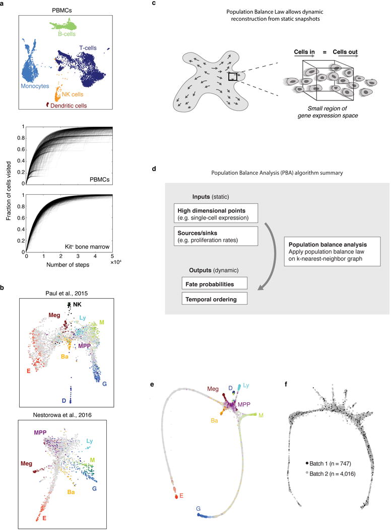
Single-cell RNA-seq of Kit+ hematopoietic progenitors for prediction of the early hematopoietic hierarchy.
a Upper panel: SPRING plot of 7,959 human peripheral blood mononuclear cells (PBMCs) from 10× Genomics [https://support.10xgenomics.com/single-cell-gene-expression/datasets/2.0.1/pbmc8k]. Clusters were generated by performing spectral clustering on the underlying k-nearest-neighbor (kNN) graph and annotated on the basis of marker genes. NK cell, natural killer cell. Middle and lower panels: Random walks over kNN graphs for the PBMC (middle) and Kit+ bone marrow (lower) datasets. Each plot shows the fraction of nodes (cells) visited for 1,000 simulated random walks.
b Left panel: SPRING plot of 2,855 lineage (Lin)−Kit+Sca1− mouse hematopoietic progenitor cells from Paul et al.12 Right: SPRING plot of 1,656 cells from three mouse hematopoietic progenitor populations (Lin−Kit+Sca1−, Lin−Kit+Sca1+, and Lin−Kit+Sca1+Flk2−CD34+) from Nestorowa et al.15 Colored (non-gray) cells indicate expression of lineage-specific genes (see Supplementary Table 7). E, erythroid; Ba, basophil/mast cell; Meg, megakaryocyte; MPP, multipotent progenitor; Ly, lymphocyte; NK, natural killer cells; M, monocyte; G, granulocyte; D, dendritic cell.
c Schematic of the Population Balance Law, which relates the dynamic velocities of cells to the distribution of states they are in at a moment in time. The law states that in steady state, after accounting for cell division and loss, the flux of cells entering any region of gene expression space equals the flux out of that region.
d Flow diagram of inputs and outputs to the Population Balance Analysis (PBA) algorithm. The population balance law is applied to inputs that include single-cell expression data and estimates of cell proliferation and loss rates at each point in gene expression space; outputs infer cell dynamics, including fate probabilities and pseudo-temporal ordering.
e SPRING plot of bone marrow Kit+ cells (Fig. 1) constructed using only the PBA-predicted fate probabilities and differentiation ordering as inputs (n= 4763 cells from one InDrops experiment). Colored cells indicate expression of lineage-specific genes as in Fig. 1b.
f SPRING plot of bone marrow Kit+ cells (Fig. 1), with cells colored by library preparation batch.
Extended Data Figure 2.
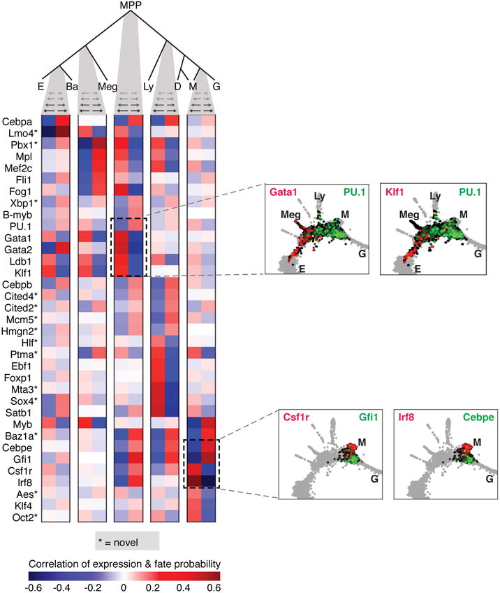
Predicting key regulators at hematopoietic choice points.
Candidate regulators of fate choice, identified by ranking transcription factors and transmembrane receptors by their correlation with PBA-predicted fate probabilities at key choice points in hematopoiesis. Top-ranked genes are shown; these include many canonical regulators. Candidates not previously reported are marked by asterisk. Several candidates participate in more than one fate choice. Insets show SPRING plots colored by expression of representative genes.
Extended Data Figure 3.
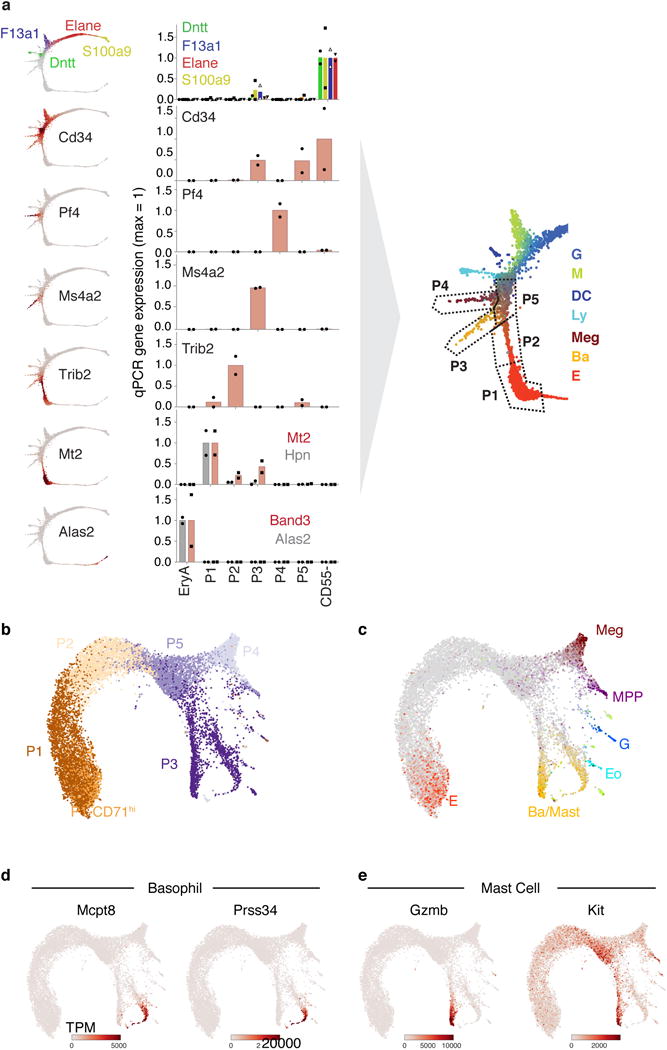
Mapping HPC subsets P1-P5 to the Kit**+ SPRING plot by RT-qPCR and scRNA-seq**
a Subpopulations P1 to P5 map onto specific regions of the SPRING plot. On the left are SPRING plot heat maps for a panel of marker genes; on the right are corresponding measured expression for each of the marker genes by RT-qPCR, performed on sorted cell subsets P1 to P5, and on EryA (= cells undergoing ETD2). A cartoon illustrates the mapping of each of P1 to P5 onto the SPRING plot based on the RT-qPCR results. Bars are mean of n= 2 independent experiment (circles, triangles or squares). Expression is shown normalized to β-actin mRNA.
b,c SPRING plot of single-cell transcriptomes from freshly sorted P1-P5 subsets (Fig. 2a–b). Cells are colored by sorted subpopulation (b) or by expression of lineage-specific marker genes (c) (Supplementary Table 7).
d,e SPRING plots of P1-P5 subset cells, colored by expression of basophil (d) and mast cell (e) marker genes. The larger cell number of cells in the P3 region of the graph resolves a split between the two lineages that was not observable in the original Kit+ dataset.
Extended Data Figure 4.
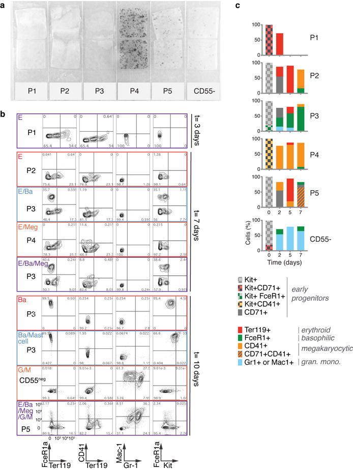
Validation of PBA predictions.
a Megakaryocytic colonies from sorted subsets P1 to P5 and from Kit+CD55− cells, stained for the megakaryocytic marker acetylcholinesterase. Duplicate cultures are shown; representative of n=2 independent experiments.
b Representative flow cytometry plots to assay fate output of single cells in liquid culture (see Fig. 3, including Fig. 3a for experimental design). Each row corresponds to a single clone, with the left column indicating the source subset (P1 to P5, CD55−) of the clone and the cell type(s) produced, as inferred from the FACS plots in the remaining columns. These data are representative of n= 1158 single cell clonal cultures, pooled from a total of n=3 independent sorting experiments (complete dataset is shown in Fig. 3b).
c Bulk liquid cultures of freshly sorted P1 to P5 subsets and Kit+CD55− cells in the presence of Epo and a cocktail of cytokines supporting myeloid progenitors. On the indicated days, cells were labeled with antibodies as indicated and analyzed by flow cytometry.
Extended Data Figure 5.
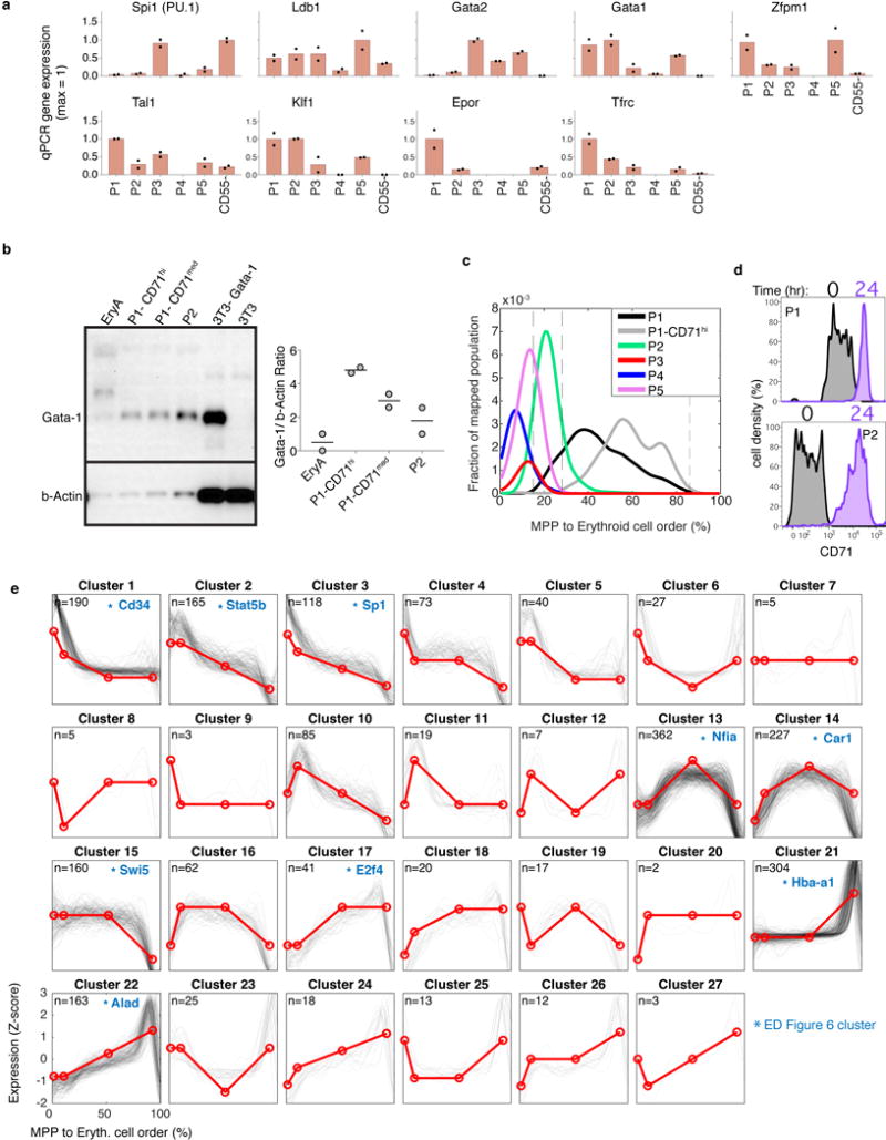
The early erythroid trajectory.
a RT-qPCR for expression of established erythroid regulators in sorted P1 to P5 subsets. Expression of each gene is normalized to β-actin, Bars are mean of n=2 independent experiments (circles).
b Left: representative western blot of GATA1 expression in sorted P1 (subdivided into CD71med and CD71hi subsets), P2, and EryA (CD71+Ter119+FSChi cells, representative of ETD). 3T3-Gata-1: 3T3 cells virally transduced with Gata-1 expression vector, used as positive control; untransduced 3T3 cells were used as negative control. Right: Quantitation of Gata-1 expression (mean) by densitometry; Data points are of two independent western blots. For gel source data, see Supplementary Figure 1.
c Density of FACS subsets P1 to P5 along the erythroid trajectory. Single-cell transcriptomes from each subset were mapped to their most similar counterparts in the Kit+ data (Fig. 2a–b; cell number analyzed for each subset are indicated in Fig. 2b). Shown here is the fraction of mapped cells, following smoothing with a Gaussian kernel. Also included are CD71High P1 cells, constituting cells with the 30% highest CD71 expression in that subset (n=752 cells post-filter).
d Distribution of CD71 expression in P1 and P2 cells immediately following sorting (gray) and after 24 hours of in vitro differentiation (lavender). Representative of n= 2 independent experiments.
e Dynamically varying genes along the MPP to erythroid axis were clustered based on their behavior across three transition points. At each transition, gene expression is either increased, decreased, or unchanged, giving a total of 27 potential dynamic patterns across all 3 transitions, shown in red. The number of genes corresponding to each dynamic pattern is noted, and individual gene Z-score normalized expression traces are shown in black. Selected clusters were further analyzed in Extended Data Figure 6 and are marked with an asterisk and a representative gene.
Extended Data Figure 6.
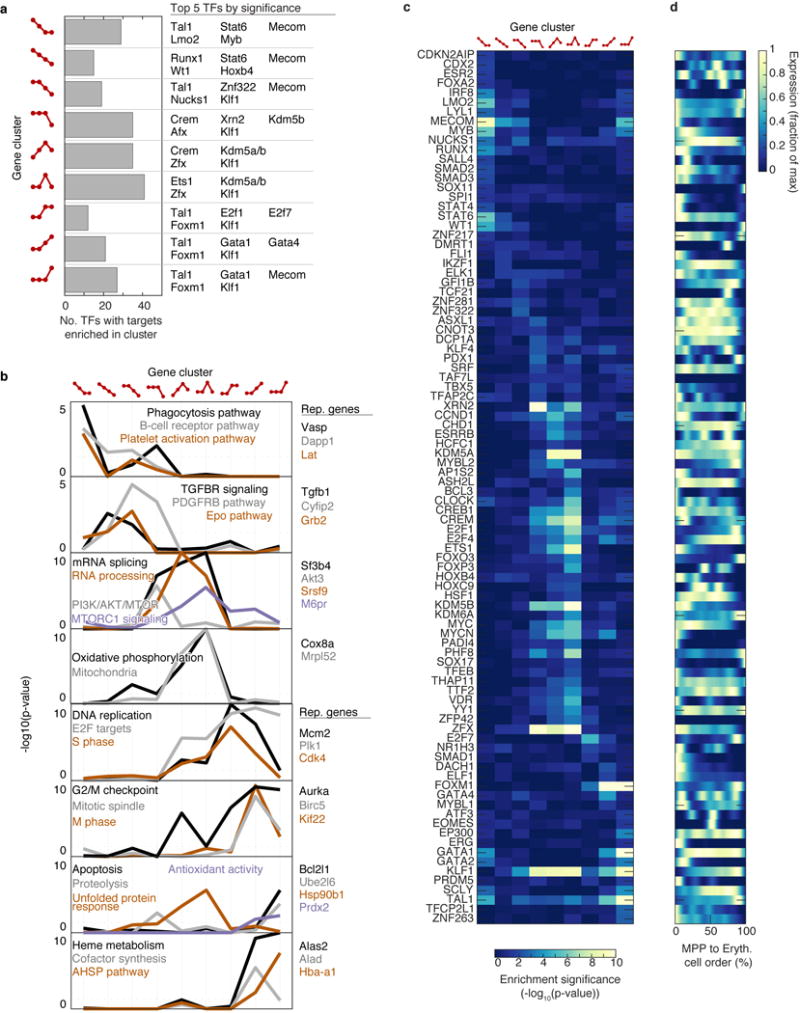
Gene set enrichment on dynamic gene clusters in early erythroid differentiation.
a-d Nine key dynamic gene clusters along the MPP to erythroid progression (Extended Data Figure 5e) are analyzed further for gene ontology. Each cluster is identified by its dynamic pattern with a cartoon of nodes and edges. Each node represents a progenitor stage (in order, MPP/EBMegP+EEP/CEP/ETD), connected to the next stage by an edge that is either going up (for increased expression) or down (for decreased expression; see Extended Data Figure 5e).
a Number and identity of transcription factors (TFs) whose targets are enriched in the dynamic clusters, as predicted by ChIP-X experiments62.
b Significance of enrichment for signaling pathways and Gene Ontology gene sets in the dynamic gene clusters (hypergeometric test with Benjamini-Hochberg correction for multiple hypothesis testing).
c,d Enrichment of transcription factor targets (TFT).
c Heatmap (−log10 of p value of hypergeometric test with Benjamini-Hochberg correction for multiple hypothesis testing) of target gene enrichment for TFs (rows) with targets significantly enriched (p<0.05) in at least one of the nine dynamic clusters (columns, labeled on top) highlighted in Extended Data Figure 5e. Note that the TFTs shown are based on previous ChIP-X experiments62 and it is possible that unappreciated TFTs occur in early erythropoiesis.
d Gene expression traces over the erythroid trajectory for the TFs from (c). Rows match those in (c).
Extended Data Figure 7. Quantification of absolute Kit+ cell number in bone-marrow following in vivo administration of Epo.
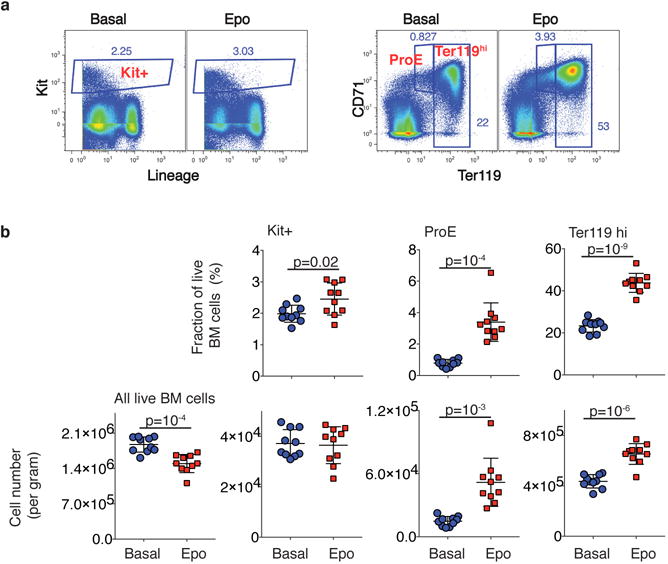
a, b Adult female mice, eight weeks of age, were injected with either Epo (100 U/25 g) or saline (=basal), once per day for two days. Bone marrow was harvested at 48 hours. Viable (trypan blue negative) cells were counted using a TC20™ automated cell counter (BIORAD) and stained for Kit, Ter119 and CD71 and lineage markers. Data is from n=two independent experiments, with 5 mice analyzed individually in each group (basal or Epo) in each experiment.
a, Representative flow cytometric analysis of either basal or Epo-stimulated bone marrow, gating on Kit+ Lin− cells (left panels) or on proerythroblasts (ProE) and Ter119hi cells (right panels; ProE and Ter119hi cells are sequential stages of ETD).
b, Data summary (mean ± SD) for all mice (n= 10 for each group). Top panels show the fraction of all BM cells for each of the flow cytometric gates defined in (a). The lower panels show the absolute cell count in adult bone marrow for subsets defined as in each flow cytometric gate, or for the total number of bone-marrow cells. P values (2-tailed t test, unequal variance) are shown for all p<0.05.
Extended Data Figure 8. Identification of stage-specific differential gene expression during the erythroid stress response.
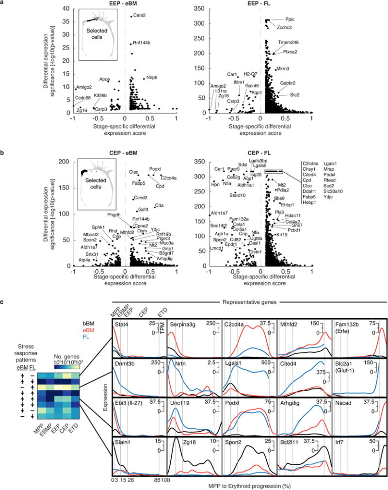
a Identification of genes differentially expressed in EEP cells of either eBM (left panel) or FL (right panel), compared with basal BM (n=1 single cell inDrop experiment per condition). P-values were calculated using a binomial test for differential expression (see Methods) and measure the significance of the expression difference. The specific enrichment score (also described in Methods) measures the degree to which the differential expression is specific to this region of interest (EEPs); positive scores correspond to region-specific upregulation, and negative to region-specific downregulation. Selected genes are highlighted.
b The same analysis applied to the CEP stage (n=1 single cell inDrop experiment per condition).
c Stage-specific differential gene expression during stress, comparing eBM and FL. The heatmap (left) shows the number of DE genes at each stage that show similar or different patterns of upregulation and downregulation in FL and eBM. Representative gene traces are shown on the right.
Extended Data Figure 9. Localized gene expression and functional response of the erythroid lineage to stimulation of Mst1, Ryk and IL-17Ra.
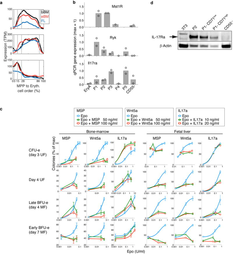
a,b Predicted expression pattern (a) and confirmation by RT-qPCR (b) for Mst1r, Ryk and Il17ra in basal BM. In (a) traces show the smoothed scRNA-Seq gene expression on cells arranged along the erythroid trajectory in basal BM, FL and eBM. RT-qPCR data are mean (bars) of n= two independent exeriments (circles).
c Complete results for CFU-e and BFU-e colony formation assays in methylcellulose, supporting the data shown in Fig. 5. Curves show colony numbers in the presence of increasing concentrations of Epo, or Epo with added ligand, either MSP, Wnt5a or IL-17a. Error bars show SD of two independent experiments, with four replicates per experiment. Where appropriate, data was fitted with a dose-response curve, Hill coefficient=1.
d Western blot shows IL-17Ra peak expression in P2/EEP cells, dropping in P1/CEP and in the granulocytic branch (which contributes most of the CD55− cells), consistent with the SPRING plots in Fig. 5a. Western blot is representative of n= two independent experiments. For gel source data, see Supplementary Figure 1.
Extended Data Figure 10. Independence of cell ordering on cell cycle genes, and evidence of an S-phase dependent CEP-to-ETD transition in BM erythropoiesis.
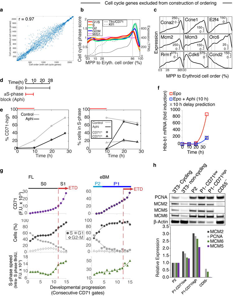
a The computational ordering of cells from MPP to ETD is not sensitive to whether or not annotated cell cycle genes are included (cell ordering correlation is R=0.97).
b,c Reproduction of main text figure panels 6b,c after excluding cell cycle genes shows that the computationally inferred gene expression dynamics of cell cycle genes during EEP/CEP differentiation are not sensitive to whether or not annotated cell cycle genes are included in ordering cells.
d-f Activation of ETD is dependent on S phase. The experiment illustrated in e-f is representative of two independent experiments.
d Schematic illustration of experiments testing the link between S-phase progression and the CEP-to-ETD transition. BM Kit+Lin−CD71− cells were cultured in the presence of Epo for 28 hours, and either in the presence or absence of the DNA polymerase inhibitor Aphidicolin (Aphi) for the first 10 hours.
e BM Kit+Lin−CD71− cells require S phase in order to upregulate CD71, an initial event in ETD. Cells were treated as in (d); left: CD71hi cells fail to appear in the first 10 hours if cells are exposed to Aphi; they appear as soon as Aphi is removed from the medium. Right: cell cycle analysis of the same cells shows that Aphi prevented S phase progression during its presence in the culture medium; Aphi removal was followed by full recovery of S phase progression, with a high fraction of CD71hi cells in S phase. Representative of n=3 independent experiments.
f Aphi exposure for 10 hours delays induction of β-globin (Hbb-b1) by 10 hours. Representative of n= 2 independent experiments.
g CD71 expression (top row), cell cycle phase distribution (middle), and intra-S phase DNA synthesis rate (lower), for consecutive FACS gates of increasing CD71 in early stages of erythropoiesis from the fetal liver (left panel, representative of n= 4 independent experiments) and Epo-simulated bone marrow (right; n=2). See Fig. 6e,f for similar analysis in basal BM.
h Western blots (upper panel) and their quantification by densitometry (lower) showing an increase in S phase proteins during progression from EEP/P2 to early CEP (P1-CD71lo to late CEP (P1-CD71hi). Controls 3T3 cells were either cycling, or contact-inhibited (non-cycling), as indicated. Western blots are representative of n=3 independent experiments. For gel source data, see Supplementary Figure 1.
Acknowledgments
This work was funded by a Leukemia and Lymphoma Society Scholar award (1728-13) and R01DK100915, R01099281 (MS). AMK is supported by a BW Fund CASI award and an Edward J Mallinckrodt Foundation Grant. SLW and CW are supported by NIH training grant 5T32GM080177-07.
Footnotes
Supplementary Information is available in the online version of the paper
Author Contributions: MS and AMK designed the experiments and supervised the project. BKT, SLW, YH, DH and RZ performed experiments including inDrops (BKT, RZ, SLW), FACS and antibody screening (BKT, DH), single cell fate assays and cell cycle analysis (BKT), Western Blotting (YH), qPCR (BTK), pSTAT3/5 (YH, DH) and colony assays for novel growth factors (YH). SLW and CW performed single cell data analysis, informatics and PBA modeling. AW and JRH provided IL17RA−/− mice. BKT, SLW, CW, YH, DH, AMK and MS prepared figures and wrote the manuscript.
Competing Interests: AMK is a co-founder of 1Cell-Bio.
References
- 1.Fujiwara Y, Browne CP, Cunniff K, Goff SC, Orkin SH. Arrested development of embryonic red cell precursors in mouse embryos lacking transcription factor GATA-1. Proc Natl Acad Sci USA. 1996;93:12355–12358. doi: 10.1073/pnas.93.22.12355. [DOI] [PMC free article] [PubMed] [Google Scholar]
- 2.Liu Y, et al. Suppression of Fas-FasL coexpression by erythropoietin mediates erythroblast expansion during the erythropoietic stress response in vivo. Blood. 2006;108:123–133. doi: 10.1182/blood-2005-11-4458. [DOI] [PMC free article] [PubMed] [Google Scholar]
- 3.Chen K, et al. Resolving the distinct stages in erythroid differentiation based on dynamic changes in membrane protein expression during erythropoiesis. Proc Natl Acad Sci U S A. 2009;106:17413–17418. doi: 10.1073/pnas.0909296106. [DOI] [PMC free article] [PubMed] [Google Scholar]
- 4.Hara H, Ogawa M. Erythropoietic precursors in mice under erythropoietic stimulation and suppression. Exp Hematol. 1977;5:141–148. [PubMed] [Google Scholar]
- 5.Gregory CJ, McCulloch EA, Till JE. The cellular basis for the defect in haemopoiesis in flexed-tailed mice. III. Restriction of the defect to erythropoietic progenitors capable of transient colony formation in vivo. Br J Haematol. 1975;30:401–410. doi: 10.1111/j.1365-2141.1975.tb01854.x. [DOI] [PubMed] [Google Scholar]
- 6.Pronk CJ, et al. Elucidation of the phenotypic, functional, and molecular topography of a myeloerythroid progenitor cell hierarchy. Cell Stem Cell. 2007;1:428–442. doi: 10.1016/j.stem.2007.07.005. doi: S1934-5909(07)00071-9[pii] 10.1016/j.stem.2007.07.005. [DOI] [PubMed] [Google Scholar]
- 7.Flygare J, Rayon Estrada V, Shin C, Gupta S, Lodish HF. HIF1alpha synergizes with glucocorticoids to promote BFU-E progenitor self-renewal. Blood. 2011;117:3435–3444. doi: 10.1182/blood-2010-07-295550. doi:blood-2010-07-295550 [pii] 10.1182/blood-2010-07-295550. [DOI] [PMC free article] [PubMed] [Google Scholar]
- 8.Li J, et al. Isolation and transcriptome analyses of human erythroid progenitors: BFU-E and CFU-E. Blood. 2014;124:3636–3645. doi: 10.1182/blood-2014-07-588806. [DOI] [PMC free article] [PubMed] [Google Scholar]
- 9.Mori Y, Chen JY, Pluvinage JV, Seita J, Weissman IL. Prospective isolation of human erythroid lineage-committed progenitors. Proc Natl Acad Sci U S A. 2015;112:9638–9643. doi: 10.1073/pnas.1512076112. 10.1073/pnas.1512076112. [DOI] [PMC free article] [PubMed] [Google Scholar]
- 10.Guo G, et al. Mapping cellular hierarchy by single-cell analysis of the cell surface repertoire. Cell Stem Cell. 2013;13:492–505. doi: 10.1016/j.stem.2013.07.017. [DOI] [PMC free article] [PubMed] [Google Scholar]
- 11.Sun J, et al. Clonal dynamics of native haematopoiesis. Nature. 2014;514:322–327. doi: 10.1038/nature13824. http://www.nature.com/nature/journal/v514/n7522/abs/nature13824.html-supplementary-information. [DOI] [PMC free article] [PubMed] [Google Scholar]
- 12.Paul F, et al. Transcriptional Heterogeneity and Lineage Commitment in Myeloid Progenitors. Cell. 2015;163:1663–1677. doi: 10.1016/j.cell.2015.11.013. [DOI] [PubMed] [Google Scholar]
- 13.Busch K, et al. Fundamental properties of unperturbed haematopoiesis from stem cells in vivo. Nature. 2015;518:542–546. doi: 10.1038/nature14242. http://www.nature.com/nature/journal/v518/n7540/abs/nature14242.html-supplementary-information. [DOI] [PubMed] [Google Scholar]
- 14.Notta F, et al. Distinct routes of lineage development reshape the human blood hierarchy across ontogeny. Science. 2016;351:aab2116. doi: 10.1126/science.aab2116. [DOI] [PMC free article] [PubMed] [Google Scholar]
- 15.Nestorowa S, et al. A single-cell resolution map of mouse hematopoietic stem and progenitor cell differentiation. Blood. 2016;128:e20–31. doi: 10.1182/blood-2016-05-716480. [DOI] [PMC free article] [PubMed] [Google Scholar]
- 16.Velten L, et al. Human haematopoietic stem cell lineage commitment is a continuous process. Nat Cell Biol. 2017;19:271–281. doi: 10.1038/ncb3493. [DOI] [PMC free article] [PubMed] [Google Scholar]
- 17.Mercier FE, Scadden DT. Not All Created Equal: Lineage Hard-Wiring in the Production of Blood. Cell. 2015;163:1568–1570. doi: 10.1016/j.cell.2015.12.013. [DOI] [PubMed] [Google Scholar]
- 18.Kondo M, Weissman IL, Akashi K. Identification of clonogenic common lymphoid progenitors in mouse bone marrow. Cell. 1997;91:661–672. doi: 10.1016/s0092-8674(00)80453-5. [DOI] [PubMed] [Google Scholar]
- 19.Akashi K, Traver D, Miyamoto T, Weissman IL. A clonogenic common myeloid progenitor that gives rise to all myeloid lineages. Nature. 2000;404:193–197. doi: 10.1038/35004599. [DOI] [PubMed] [Google Scholar]
- 20.Adolfsson J, et al. Identification of Flt3+ lympho-myeloid stem cells lacking erythro-megakaryocytic potential a revised road map for adult blood lineage commitment. Cell. 2005;121:295–306. doi: 10.1016/j.cell.2005.02.013. doi:S0092-8674(05)00158-3 [pii] 10.1016/j.cell.2005.02.013. [DOI] [PubMed] [Google Scholar]
- 21.Huang W, Cao X, Biase FH, Yu P, Zhong S. Time-variant clustering model for understanding cell fate decisions. Proceedings of the National Academy of Sciences. 2014;111:E4797–E4806. doi: 10.1073/pnas.1407388111. [DOI] [PMC free article] [PubMed] [Google Scholar]
- 22.Marco E, et al. Bifurcation analysis of single-cell gene expression data reveals epigenetic landscape. Proceedings of the National Academy of Sciences. 2014;111:E5643–E5650. doi: 10.1073/pnas.1408993111. [DOI] [PMC free article] [PubMed] [Google Scholar]
- 23.Shin J, et al. Single-Cell RNA-Seq with Waterfall Reveals Molecular Cascades underlying Adult Neurogenesis. Cell Stem Cell. 2015;17:360–372. doi: 10.1016/j.stem.2015.07.013. doi: https://doi.org/10.1016/j.stem.2015.07.013. [DOI] [PMC free article] [PubMed] [Google Scholar]
- 24.Ji Z, Ji H. TSCAN: Pseudo-time reconstruction and evaluation in single-cell RNA-seq analysis. Nucleic Acids Research. 2016;44:e117–e117. doi: 10.1093/nar/gkw430. [DOI] [PMC free article] [PubMed] [Google Scholar]
- 25.Welch JD, Hartemink AJ, Prins JF. SLICER: inferring branched, nonlinear cellular trajectories from single cell RNA-seq data. Genome Biology. 2016;17:106. doi: 10.1186/s13059-016-0975-3. [DOI] [PMC free article] [PubMed] [Google Scholar]
- 26.Haghverdi L, Buttner M, Wolf FA, Buettner F, Theis FJ. Diffusion pseudotime robustly reconstructs lineage branching. Nat Meth. 2016;13:845–848. doi: 10.1038/nmeth.3971. http://www.nature.com/nmeth/journal/v13/n10/abs/nmeth.3971.html-supplementary-information. [DOI] [PubMed] [Google Scholar]
- 27.Moignard V, et al. Decoding the regulatory network of early blood development from single-cell gene expression measurements. Nat Biotech. 2015;33:269–276. doi: 10.1038/nbt.3154. http://www.nature.com/nbt/journal/v33/n3/abs/nbt.3154.html-supplementary-information. [DOI] [PMC free article] [PubMed] [Google Scholar]
- 28.Arnold LW, Lannigan J. Current Protocols in Cytometry. John Wiley & Sons, Inc; 2001. [Google Scholar]
- 29.Klein AM, et al. Droplet barcoding for single-cell transcriptomics applied to embryonic stem cells. Cell. 2015;161:1187–1201. doi: 10.1016/j.cell.2015.04.044. [DOI] [PMC free article] [PubMed] [Google Scholar]
- 30.Morrison SJ, Weissman IL. The long-term repopulating subset of hematopoietic stem cells is deterministic and isolatable by phenotype. Immunity. 1994;1:661–673. doi: 10.1016/1074-7613(94)90037-x. [DOI] [PubMed] [Google Scholar]
- 31.Papayannopoulou T, Brice M, Broudy V, Zsebo K. Isolation of c-kit receptor-expressing cells from bone marrow, peripheral blood, and fetal liver: functional properties and composite antigenic profile. Blood. 1991;78:1403–1412. [PubMed] [Google Scholar]
- 32.Weinreb C, Wolock S, Klein A. SPRING: a kinetic interface for visualizing high dimensional single-cell expression data. Bioinformatics. 2017 doi: 10.1093/bioinformatics/btx792. [DOI] [PMC free article] [PubMed] [Google Scholar]
- 33.Weinreb C, Wolock S, Khoramian Tusi B, Socolovsky M, Klein AM. Fundamental limits on dynamic inference from single cell snapshots. BioRxiv. 2017;170118 doi: 10.1073/pnas.1714723115. [DOI] [PMC free article] [PubMed] [Google Scholar]
- 34.Yanez A, et al. Granulocyte-Monocyte Progenitors and Monocyte-Dendritic Cell Progenitors Independently Produce Functionally Distinct Monocytes. Immunity. 2017;47:890–902 e894. doi: 10.1016/j.immuni.2017.10.021. [DOI] [PMC free article] [PubMed] [Google Scholar]
- 35.Magwene PM, Lizardi P, Kim J. Reconstructing the temporal ordering of biological samples using microarray data. Bioinformatics. 2003;19:842–850. doi: 10.1093/bioinformatics/btg081. [DOI] [PubMed] [Google Scholar]
- 36.Bendall SC, et al. Single-cell trajectory detection uncovers progression and regulatory coordination in human B cell development. Cell. 2014;157:714–725. doi: 10.1016/j.cell.2014.04.005. [DOI] [PMC free article] [PubMed] [Google Scholar]
- 37.Trapnell C, et al. The dynamics and regulators of cell fate decisions are revealed by pseudotemporal ordering of single cells. Nat Biotechnol. 2014;32:381–386. doi: 10.1038/nbt.2859. [DOI] [PMC free article] [PubMed] [Google Scholar]
- 38.Bresnick EH, Lee HY, Fujiwara T, Johnson KD, GATA Keles S. Switches as Developmental Drivers. Journal of Biological Chemistry. 2010;285:31087–31093. doi: 10.1074/jbc.R110.159079. [DOI] [PMC free article] [PubMed] [Google Scholar]
- 39.Li P, et al. Regulation of bone marrow hematopoietic stem cell is involved in high-altitude erythrocytosis. Experimental Hematology. 2011;39:37–46. doi: 10.1016/j.exphem.2010.10.006. [DOI] [PubMed] [Google Scholar]
- 40.Grover A, et al. Erythropoietin guides multipotent hematopoietic progenitor cells toward an erythroid fate. J Exp Med. 2014;211:181–188. doi: 10.1084/jem.20131189. [DOI] [PMC free article] [PubMed] [Google Scholar]
- 41.Mancini E, et al. FOG-1 and GATA-1 act sequentially to specify definitive megakaryocytic and erythroid progenitors. EMBO J. 2012;31:351–365. doi: 10.1038/emboj.2011.390. [DOI] [PMC free article] [PubMed] [Google Scholar]
- 42.Koulnis M, Porpiglia E, Hidalgo D, Socolovsky MI. In: A Systems Biology Approach to Blood Vol. 844 Advances in Experimental Medicine and Biology. Corey Seth Joel, Kimmel Marek, Leonard Joshua N., editors. Springer; New York: 2014. pp. 37–58. Ch. 3. [DOI] [PubMed] [Google Scholar]
- 43.Agosti V, Karur V, Sathyanarayana P, Besmer P, Wojchowski DM. A KIT juxtamembrane PY567 -directed pathway provides nonredundant signals for erythroid progenitor cell development and stress erythropoiesis. Exp Hematol. 2009;37:159–171. doi: 10.1016/j.exphem.2008.10.009. doi:S0301-472X(08)00483-9 [pii] 10.1016/j.exphem.2008.10.009. [DOI] [PMC free article] [PubMed] [Google Scholar]
- 44.Koury MJ, Bondurant MC. Erythropoietin retards DNA breakdown and prevents programmed death in erythroid progenitor cells. Science. 1990;248:378–381. doi: 10.1126/science.2326648. [DOI] [PubMed] [Google Scholar]
- 45.Yee K, Bishop TR, Mather C, Zon LI. Isolation of a novel receptor tyrosine kinase cDNA expressed by developing erythroid progenitors. Blood. 1993;82:1335–1343. [PubMed] [Google Scholar]
- 46.van den Akker E, et al. Tyrosine kinase receptor RON functions downstream of the erythropoietin receptor to induce expansion of erythroid progenitors. Blood. 2004;103:4457–4465. doi: 10.1182/blood-2003-08-2713. [DOI] [PubMed] [Google Scholar]
- 47.Pop R, et al. A key commitment step in erythropoiesis is synchronized with the cell cycle clock through mutual inhibition between PU.1 and S-phase progression. PLoS Biol. 2010;8 doi: 10.1371/journal.pbio.1000484. [DOI] [PMC free article] [PubMed] [Google Scholar]
- 48.Hwang Y, et al. Global increase in replication fork speed during a p57KIP2-regulated erythroid cell fate switch. Science Advances. 2017;3:e1700298. doi: 10.1126/sciadv.1700298. [DOI] [PMC free article] [PubMed] [Google Scholar]
- 49.Shearstone JR, et al. Global DNA demethylation during mouse erythropoiesis in vivo. Science. 2011;334:799–802. doi: 10.1126/science.1207306. doi: 334/6057/799[pii] 10.1126/science.1207306. [DOI] [PMC free article] [PubMed] [Google Scholar]
- 50.Nemeth E, Ganz T. Anemia of Inflammation. Hematology/Oncology Clinics of North America. 2014;28:671–681. doi: 10.1016/j.hoc.2014.04.005. doi: https://doi.org/10.1016/j.hoc.2014.04.005. [DOI] [PMC free article] [PubMed] [Google Scholar]
- 51.Liang R, et al. A Systems Approach Identifies Essential FOXO3 Functions at Key Steps of Terminal Erythropoiesis. PLOS Genetics. 2015;11:e1005526. doi: 10.1371/journal.pgen.1005526. [DOI] [PMC free article] [PubMed] [Google Scholar]
- 52.Whitfield ML, et al. Identification of genes periodically expressed in the human cell cycle and their expression in tumors. Mol Biol Cell. 2002;13:1977–2000. doi: 10.1091/mbc.02-02-0030.. [DOI] [PMC free article] [PubMed] [Google Scholar]
Additional References for Methods section
- 53.Zilionis R, et al. Single-cell barcoding and sequencing using droplet microfluidics. Nat Protocols. 2017;12:44–73. doi: 10.1038/nprot.2016.154. http://www.nature.com/nprot/journal/v12/n1/abs/nprot.2016.154.html-supplementary-information. [DOI] [PubMed] [Google Scholar]
- 54.Ester M, Kriegel H, Sander J, Xu XI. Conf on Knowledge Discovery and Data Mining. :226. [Google Scholar]
- 55.Daszykowski M, Walczak B, Massart DL. Looking for natural patterns in data: Part 1. Density-based approach. Chemometrics and Intelligent Laboratory Systems. 2001;56:83–92. doi: http://dx.doi.org/10.1016/S0169-7439(01)00111-3. [Google Scholar]
- 56.van der Maaten L. Accelerating t-SNE using Tree-Based Algorithms. Journal of Machine Learning Research. 2014;15:3221–3245. [Google Scholar]
- 57.Macosko EZ, et al. Highly Parallel Genome-wide Expression Profiling of Individual Cells Using Nanoliter Droplets. Cell. 2015;161:1202–1214. doi: 10.1016/j.cell.2015.05.002. [DOI] [PMC free article] [PubMed] [Google Scholar]
- 58.Weinreb C, Wolock S, Klein AM. SPRING: a kinetic interface for visualizing high dimensional single-cell expression data. BioRxiv. 2017:090332. doi: 10.1093/bioinformatics/btx792. [DOI] [PMC free article] [PubMed] [Google Scholar]
- 59.Vandin F, Upfal E, Raphael BJ. Algorithms for detecting significantly mutated pathways in cancer. J Comput Biol. 2011;18:507–522. doi: 10.1089/cmb.2010.0265. [DOI] [PubMed] [Google Scholar]
- 60.Heng TS, Painter MW, Immunological Genome Project, C The Immunological Genome Project: networks of gene expression in immune cells. Nat Immunol. 2008;9:1091–1094. doi: 10.1038/ni1008-1091. [DOI] [PubMed] [Google Scholar]
- 61.Subramanian A, et al. Gene set enrichment analysis: a knowledge-based approach for interpreting genome-wide expression profiles. Proc Natl Acad Sci U S A. 2005;102:15545–15550. doi: 10.1073/pnas.0506580102. [DOI] [PMC free article] [PubMed] [Google Scholar]
- 62.Lachmann A, et al. ChEA: transcription factor regulation inferred from integrating genome-wide ChIP-X experiments. Bioinformatics. 2010;26:2438–2444. doi: 10.1093/bioinformatics/btq466. [DOI] [PMC free article] [PubMed] [Google Scholar]
- 63.Scialdone A, et al. Computational assignment of cell-cycle stage from single-cell transcriptome data. Methods. 2015;85:54–61. doi: 10.1016/j.ymeth.2015.06.021. [DOI] [PubMed] [Google Scholar]
- 64.Santos A, Wernersson R, Jensen LJ. Cyclebase 3.0: a multi-organism database on cell-cycle regulation and phenotypes. Nucleic Acids Res. 2015;43:D1140–1144. doi: 10.1093/nar/gku1092. [DOI] [PMC free article] [PubMed] [Google Scholar]
- 65.Shekhar K, et al. Comprehensive Classification of Retinal Bipolar Neurons by Single-Cell Transcriptomics. Cell. 2016;166:1308–1323 e1330. doi: 10.1016/j.cell.2016.07.054. [DOI] [PMC free article] [PubMed] [Google Scholar]
- 66.Benjamini Y, Hochberg Y. Controlling the false discovery rate: a practical and powerful approach to multiple testing. Journal of the Royal Statistical Society, B. 1995;57:289–300. [Google Scholar]
- 67.Tusi BK, Socolovsky M. Novel FACS strategy for identification of early hematopoietic progenitors including BFU-e, CFU-e and erythroid-biased MPPs. Protocol Exchange. 2018 doi: https://www.nature.com/protocolexchange/protocols/6499.
- 68.El Malki K, et al. An Alternative Pathway of Imiquimod-Induced Psoriasis-Like Skin Inflammation in the Absence of Interleukin-17 Receptor A Signaling. Journal of Investigative Dermatology. 2013;133:441–451. doi: 10.1038/jid.2012.318. doi: http://dx.doi.org/10.1038/jid.2012.318. [DOI] [PubMed] [Google Scholar]
- 69.Porpiglia E, Hidalgo D, Koulnis M, Tzafriri AR, Socolovsky M. Stat5 signaling specifies basal versus stress erythropoietic responses through distinct binary and graded dynamic modalities. PLoS Biol. 2012;10:e1001383. doi: 10.1371/journal.pbio.1001383. 10.1371/journal.pbio.1001383 PBIOLOGY-D-12-00220 [pii] [DOI] [PMC free article] [PubMed] [Google Scholar]
Associated Data
This section collects any data citations, data availability statements, or supplementary materials included in this article.
Supplementary Materials
Supplementary information guide, Supplementary Tables 1, 2, 7, Source data for gels
Supplementary Table 3
Supplementary Table 4
Supplementary Table 5
Supplementary Table 6
Source data for Extended Data Figure 10
Source data for Figure 2c-e
Source Data for Extended Data Figure 3a
Source Data for Extended Data Figure 4c
Source Data for Extended Data Figure 5a-b
Source Data for Figure 6f
Source Data for Extended Data Figure 7b
Source Data for Extended Data Figure 9b
Source Data for Figure 5b-d
Source Data for Figure 3b
PBA inputs
Data Availability Statement
Sequence data that supports the findings of this study have been deposited in the Gene Expression Omnibus (GEO, https://www.ncbi.nlm.nih.gov/geo/), accession code GSE89754. An interactive tool for these data is available at kleintools.hms.harvard.edu/paper_websites/tusi_et_al.
Source data files are provided for graphical representations in Figures 2c–e, 3b,5b–d, 6f, Extended Data Figures 3a, 4c, 5a–b, 7b, 9b, 10e, f-h; and for all immunoblots (supplementary Figure 1).