Impact of Correlated Synaptic Input on Output Firing Rate and Variability in Simple Neuronal Models (original) (raw)
Abstract
Cortical neurons are typically driven by thousands of synaptic inputs. The arrival of a spike from one input may or may not be correlated with the arrival of other spikes from different inputs. How does this interdependence alter the probability that the postsynaptic neuron will fire? We constructed a simple random walk model in which the membrane potential of a target neuron fluctuates stochastically, driven by excitatory and inhibitory spikes arriving at random times. An analytic expression was derived for the mean output firing rate as a function of the firing rates and pairwise correlations of the inputs. This stochastic model made three quantitative predictions. (1) Correlations between pairs of excitatory or inhibitory inputs increase the fluctuations in synaptic drive, whereas correlations between excitatory–inhibitory pairs decrease them. (2) When excitation and inhibition are fully balanced (the mean net synaptic drive is zero), firing is caused by the fluctuations only. (3) In the balanced case, firing is irregular. These theoretical predictions were in excellent agreement with simulations of an integrate-and-fire neuron that included multiple conductances and received hundreds of synaptic inputs. The results show that, in the balanced regime, weak correlations caused by signals shared among inputs may have a multiplicative effect on the input-output rate curve of a postsynaptic neuron, i.e. they may regulate its gain; in the unbalanced regime, correlations may increase firing probability mainly around threshold, when output rate is low; and in all cases correlations are expected to increase the variability of the output spike train.
Keywords: random-walk, integrate-and-fire, computer simulation, spike synchrony, oscillations, cross-correlation, balanced inhibition, cerebral cortex
The output of a typical cortical neuron depends on the activity of a large number of synaptic inputs—several thousands of them, as estimated by anatomical techniques (White, 1989; Braitenberg and Shüz, 1997). What kind of response should be expected from a postsynaptic neuron driven by so many inputs? Answering this question in detail requires a deep understanding of dendritic integration, synaptic function, and spike generation mechanisms; but, given the large numbers commonly involved, as a first approximation it is natural to cast the problem in statistical terms. The strategy then is to compute the output responses of a model neuron (or their statistics), given a set of driving inputs with known statistical properties. These inputs may be either independent or temporally correlated. In the latter case, spikes from different input neurons arrive close together in time more often or less often than expected by chance.
In general, the situation with independent inputs is easier to analyze, and for many applications it is probably a good approximation. However, there are at least three reasons why the effects of correlations on single cells should be fully characterized. First, correlations in spike counts have indeed been observed (Gawne and Richmond, 1993; Zohary et al., 1994; Salinas et al., 2000) and, based on the convergent connectivity of the cortex (White, 1989; Braitenberg and Schüz, 1997), they must be ubiquitous (Shadlen and Newsome, 1998; Bair et al., 1999). Second, such correlations may alter the coding capacity of a neuronal population (Gawne and Richmond, 1993; Zohary et al., 1994; Abbott and Dayan, 1999). Third, synchrony and oscillations, two forms of correlated activity that have been intensely studied, may also be important for information encoding (DeCharms and Merzenich, 1995; Riehle et al., 1997; Dan et al., 1998) or for other aspects of cortical function (Engel et al., 1992; Singer and Gray, 1995). This paper, however, does not focus on the possible higher-level functional roles of coordinated spike firing; instead, it addresses a more elementary problem: how does a typical cortical neuron react to synaptic inputs that are correlated, compared to synaptic inputs that are uncorrelated?
This problem has been investigated in the past (Bernander et al., 1994; Murthy and Fetz, 1994; Shadlen and Newsome, 1998), but the model neurons used earlier have often been examined with limited sets of parameters, and sometimes in regimes outside the normal operating range of cortical neurons; for instance, some studies have ignored the effects of inhibition. This study attempts to provide a broad framework within which the impact of input correlations on a single postsynaptic neuron can be better understood. Using a simple theoretical model, the mean firing rate of a postsynaptic neuron is solved as a function of the firing rates and pairwise correlations of its excitatory and inhibitory inputs. This model also provides qualitative insight on how correlations affect output variability. The analytic expressions are then compared to computer simulations of a conductance-based model neuron with more realistic dynamics. We find that correlations affect both the firing rate and variability of the output and that the strength and details of these effects depend strongly on the balance between excitation and inhibition.
MATERIALS AND METHODS
_A theoretical model with random walk dynamics._Consider a simple stochastic model neuron in which an incoming excitatory spike increases the membrane potential by an amount ΔE, and each incoming inhibitory spike decreases the membrane potential by an amount ΔI. These voltage steps are fixed, and are independent of the input statistics. In the absence of synaptic input, the voltage of the model neuron, termed V , decreases by a fixed amount d in each time step, but there is a fixed minimum Vrest below which the voltage cannot be driven, even if inhibition is strong. The d term makes the voltage decrease linearly with time toward Vrest. Because of leak currents, membrane potentials of real neurons actually relax exponentially to their rest values, but approximating this with a linear term may be reasonable when V remains relatively far from rest. In addition, whenever the voltage exceeds a threshold Vθ, an action potential is fired, and the voltage is instantaneously reset to the value Vreset. Given specific values for these six parameters, the output of the model neuron will be entirely determined by the statistics of the inputs. The advantage of these simple dynamics is that, if the input statistics are known and certain simplifying assumptions are made, then the output firing rate may be computed analytically, revealing the explicit dependence on the input statistics. This is shown in the following sections.
The analysis follows in the tradition of classic results from the theory of stochastic processes (Ricciardi, 1977;Tuckwell, 1989; Risken, 1996). Many of the previous studies that applied these random walk methods to the problem of synaptic integration were aimed at understanding, in terms of a simple mechanistic explanation, how spike firing in a neuron is triggered by the stochastic fluctuations of its membrane potential (Tuckwell, 1988; Smith, 1992). In other studies the goal was to develop models that could account in detail for the measured firing statistics of real neurons (Gerstein and Mandelbrot, 1964; Shinomoto et al., 1999). As shown below, this framework is also of heuristic value to the problem of input correlations and their impact on firing probability (Feng and Brown, 2000).
RESULTS
Changes in voltage modeled as random walk steps
According to the above description, at each time step Δt the voltage jumps by an amount:
| ΔV=nEΔE−nIΔI−d, | Equation 1 |
|---|
where nE and nI are the total numbers of incoming excitatory and inhibitory spikes that arrived in that interval Δt . By defining the net number of excitatory spikes as:
| n≡ΔVΔE=nE−ΔIΔEnI−dΔE, | Equation 2 |
|---|
the change in voltage can be written as:
The net number of excitatory spikes will vary randomly from one time step to the next. The chance of n having a given specific value at any particular time step is characterized by the probability distribution P(n) , such that μ = 〈n〉 and ς2 = 〈(n − μ)2〉 correspond, respectively, to the mean and variance of n . Throughout the paper, angle brackets are used to indicate an average over time steps. A positive value of μ indicates a mean excess of excitatory drive versus inhibitory drive in each Δt , whereas ς represents the fluctuations in the drive. Because changes in voltage are proportional to n, V will be linearly related to the net number of excitatory spikes that have accumulated since the last output spike was emitted:
| N=Nrest+V−VrestΔE. | Equation 4 |
|---|
Thus, N changes by n in each time step, it has a lower limit of Nrest, it needs to reach a critical value Nθ for the postsynaptic neuron to fire again, and is reset to Nreset after each postsynaptic spike. Nθ is obtained when V = Vθ in the above equation, and the same is true for the other values specified by their subscripts. For convenience we will set Nrest = 0 ; this choice does not alter the results in any significant way, because what counts is the difference between N and Nθ.
Given that in each time step N changes by a random amount, N (and therefore V ) is equivalent to the net displacement of a one-dimensional random walk process with drift in which there is a reflecting barrier at one end and an absorbing barrier at the other. What we want to know is the average number of steps ν that it takes for N to go from reset to threshold. This is the same as asking how much time it typically takes for V to go from Vreset to Vθ. The total amount of time will be:
This is the mean interspike interval of the output neuron. For a random walk, this time is known as the mean time to capture (Berg, 1993). This, or its reciprocal, the mean firing rate rout, can be computed making some assumptions about the probability distribution of n . The derivation is left for the , but the main intuition is this: on average, in each time step the net change in N is μ. If ς is small, ν should be approximately Nθ/μ . Now suppose instead that μ = 0 so there is no drift. In this case N just fluctuates around its initial value. After ν steps, however, the typical displacement (positive or negative, in the root mean square sense) relative to the starting point is ςν(Feynman et al., 1963). Hence, now it should take on the order of (Nθ/ς)2 steps for N to reach a point Nθ units away. In general, then, it would seem that either μ or ς may drive the neuron to fire. A more detailed analysis confirms this idea and leads to the following expressions (see ). When μ ≥ 0 ,
| rout2Δt2((Nθ+ς)2−Nreset2)−routΔt(2μNreset+ς2)−μ2=0. | Equation 6 |
|---|
When μ > 0 there is a net excitatory drive and, in general, both μ and ς tend to increase the firing rate, although this is not true for all combinations of these two parameters. This solution is not exact, but it should be quite good as long as ς remains smaller than Nθ (see ). On the other hand, when μ ≤ 0 ,
| rout=(ς+cμ)2Δt(Nθ+ς+cμ)2−Nreset, | Equation 7 |
|---|
where c is a constant. In this case the negative drive acts to effectively decrease ς by an amount proportional to μ. This happens up to the point where ς + cμ = 0 , beyond which the output firing rate is set to zero (otherwise, ς + cμ would correspond to a negative effective SD). This approximation is partly based on simulation results shown below, where it is discussed further.
Equations 6 and 7 are useful for three reasons. First, they are valid for small and large ς (small or large relative to the distance from rest to threshold), second, they combine μ and ς seamlessly, in the sense that cases with and without drift also fall under the same formulation, and third, the approximations are best when the underlying distribution P(n) is Gaussian but they are quite good even when the distribution is very different. Other theoretical models are usually restricted in one or more of these ways (Gerstein and Mandelbrot, 1964; Tuckwell, 1988; Smith, 1992). The rest of the paper examines the behavior of these expressions: first, as functions of μ and ς, second, as functions of the mean firing rate and variability of the input spike trains, which determine μ and ς, and finally, in comparison to simulations of a more realistic, conductance-based model.
Robustness of the random walk approximations
A crucial assumption underlying the above results was that the full probability distribution of n could be represented by its mean and SD. How good is this approximation? We explored this through computer simulations in which, at each time step, n was drawn from a specified distribution, using a random number generator (Press et al., 1992). Each simulation cycle started with N = Nreset. Then, in each step, the update rule N → N + n was applied until N reached the threshold value, in which case the total number of steps elapsed was saved, and a new cycle was started. This was repeated 5000 times, after which the average number of steps ν was obtained. For the results shown in Figure1c–h, Nθ = 40, Nreset = 20 , and ς varies along the x axes. The different curves in Figure 1c–h correspond to different values of μ. The insets depict the type of distribution function for n used in the corresponding panels. The dots indicate the simulation results, and the continuous lines in Figure 1c are the analytic approximations given by Equations 6 and 7; these are the same regardless of the distribution. The analytic results are most accurate when n is distributed in a Gaussian fashion, but the random walk approximation is qualitatively accurate when the distribution of n is uniform (Fig. 1d), and even when it is sharply skewed (Fig. 1e). The approximations are good even when ς is almost as large as Nθ.
Fig. 1.
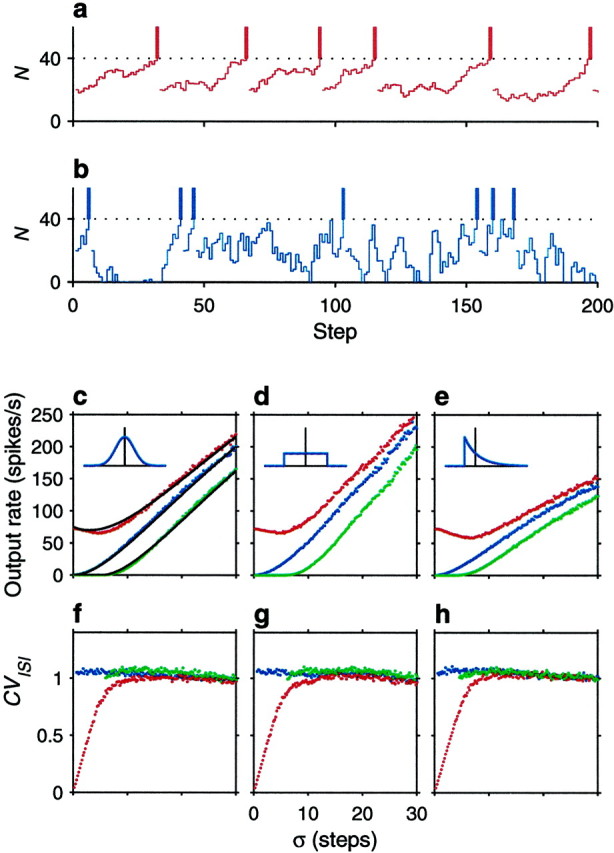
Computer simulations of the stochastic neuron model. The two traces on the top illustrate how the accumulated number of net excitatory spikes, N , varies over time. In each time step, N changes to N + n , where n is drawn from a distribution with mean μ and SD ς. When N reaches the threshold (dotted line), a spike is emitted (vertical bars), and N is lowered to its reset value. In this figure Nθ = 40 and Nreset = 20 . a, Drift dominates over the fluctuations, so the neuron fires regularly; n was drawn from a Gaussian distribution with μ = 0.71, ς = 2 . b, The neuron is driven exclusively by the fluctuations, so it fires irregularly; n was drawn from a Gaussian distribution with μ = 0, ς = 8 . Notice N cannot fall below the reflecting barrier at 0.c–e, Output firing rate (rout) as a function of ς. Red dots correspond to μ = 1.5 , blue dots_to μ = 0 , and green dots to μ = −3 . Insets indicate the distribution of n in each case; vertical lines mark the mean values. Gaussian, uniform, and exponential distributions were tested. The_continuous lines in c are the analytic results from Equations 6 and 7. f–h, Coefficient of variation of the output interspike intervals as a function of ς. The three panels correspond to the three distributions for n shown in the above insets. Colors indicate same parameter values as in panels above.
Through these simulations we also investigated what happens when N relaxes exponentially to its rest value. In this case the simulations proceeded exactly as described above, except that the update rule for N was N → hN + n , where h is a constant <1 ( h = 1 is the original case without exponential decay). This is equivalent to having a leak term proportional to −V in Equation 1 instead of the constant d . We found that the shapes of the resulting curves were very similar to those obtained using the linear decay term that contributes to μ (Eq. 2), except that they corresponded to more negative values of μ. For instance, the results of a simulation with h = 0.95 and μ = 0 were almost identical to the results obtained with h = 1 and μ = −1 . Therefore, the exact shape of the distribution of n and the precise way in which V relaxes to rest do not affect the results qualitatively.
Two output modes: mean excitatory drive versus fluctuations
The dynamics of the output neuron may be understood intuitively in the two limits mentioned before, when the drift is positive and much larger than the fluctuations, and when the drift is zero (Troyer and Miller, 1997). If the net drive is positive and ς is close to 0 (Gerstein and Mandelbrot, 1964; Tuckwell, 1988; Usher et al., 1994; Koch, 1999), Equation 6 is reduced to
| rout≈μΔt(Nθ−Nreset). | Equation 8 |
|---|
In this case rout depends linearly on the average drive, which brings V closer to threshold. Fluctuations produce some jitter in the path from rest to threshold (Tuckwell, 1988; Koch, 1999), but the interspike intervals of the model neuron should be rather regular. Figure 1a shows that this is indeed what happens. Here an individual sequence of N values from one of the simulations is shown; for this we set μ = 0.71 and ς = 2 . The trajectories from reset to threshold are similar because they are dominated by the constant drift, producing fairly regular interspike intervals.
Previous stochastic models arrived at the above expression regarding μ as the sole contributor to the mean firing rate (Gerstein and Mandelbrot, 1964; Tuckwell, 1988;Usher et al., 1994). In these models the fluctuations were considered so small relative to the distance from reset to threshold, that, in the absence of drift, it took an infinite amount of time for V to reach threshold. In the present model, however, fluctuations are not infinitesimal (Feynman et al., 1963) so, when μ = 0 ,
| rout=ς2Δt(Nθ+ς)2−Nreset2. | Equation 9 |
|---|
In this case the output firing rate increases monotonically with ς up to the limit 1/Δt . The Δt of the model has a functional interpretation: it represents the refractory period, because only one spike is allowed per Δt . In this mode the neuron fires because there are fluctuations in the numbers of excitatory and inhibitory input spikes that arrive per Δt , even though on average excitatory and inhibitory contributions balance each other out (Smith, 1992; Shadlen and Newsome, 1995; Bell et al., 1995). If the fluctuations are large, the average drive may even be negative, and this will not prevent the neuron from firing. As mentioned above, when μ is negative, the output firing rate can be accurately approximated by Equation 7, which was used in Figure 1c (continuous line over green dots). We found that c = 1.7 fitted the simulation results fairly well. In Figures 1c–e the curves for negative μ are very much like shifted versions of the curves with μ = 0 , which is precisely why the approximation works.
When the postsynaptic neuron is driven by fluctuations, the interspike interval distribution of the evoked spike trains is expected to be wide, because it follows an entirely stochastic process. As shown in Figure 1b, individual trajectories of N are widely different—they are also independent, and this produces highly variable interspike intervals. The two dynamical modes described by Equations 8 and 9 are thus distinct.
Figure 1f–h quantifies the variability of the interspike intervals produced by the simulations. The y axes indicate the coefficient of variation of the interspike interval distribution, or CVISI. This is equal to the SD of the interspike intervals divided by their mean and is shown as a function of ς using the same results used in Figure 1c–e. The plots confirm the intuitive picture discussed in the previous paragraphs: when ς is large in relation to μ, the coefficient of variation is close to 1, as expected from a Poisson process. On the other hand, as ς approaches 0, μ becomes relatively large, and the variability in the interspike intervals decreases sharply (Fig.1f–h, red dots). This drop in variability has been viewed as support for a large ς in real cortical neurons, that is, as evidence of a balance between excitation and inhibition (Shadlen and Newsome, 1994; Troyer and Miller, 1997).
Impact of input correlations
Now we quantify how the relative magnitudes of the fluctuations and the mean of the total synaptic drive may change according to the synaptic input statistics.
Assume that the model neuron receives ME and MI excitatory and inhibitory inputs, respectively. We denote the number of spikes fired by excitatory input j in a time step Δt as nEj; analogously, nIk corresponds to the number of spikes fired by inhibitory neuron k . Recalling that nE and nI are the total numbers of excitatory and inhibitory spikes, Equation 2 can be written as:
| n=∑jME nEj−ΔIΔE ∑kMI nIk−dΔE. | Equation 10 |
|---|
We are interested in the mean and the variance of n , which are μ and ς2. To calculate them, we assume that all excitatory inputs fire at the same mean rate rE, such that the average number of spikes per time step fired by any excitatory neuron is:
Similarly, all inhibitory neurons fire at a mean rate rI but, furthermore, we will assume that inhibitory and excitatory rates are proportional, such that:
| 〈nIk〉=rIΔt=αrEΔt, | Equation 12 |
|---|
where α is the constant of proportionality. With these definitions, the mean value of n is simply:
| μ=〈n〉=rEΔt ME1−αMIME ΔIΔE −dΔE. | Equation 13 |
|---|
The fraction inside the square brackets reflects the balance between excitation and inhibition,
| βRW≡αMIME ΔIΔE. | Equation 14 |
|---|
An analogous quantity is defined below (Eq. 29) for more realistic neurons. They differ because, in the random walk model, the effect of each input spike is characterized by a single, instantaneous voltage step. When βRW = 1 the neuron is fully balanced, and the mean drift in voltage attributable to synaptic inputs is zero. Notice, however, that μ in Equation 13 includes another negative term caused by leakage that is independent of the balance.
To compute the variance of n , we need to specify the variance of the individual inputs as well as their pairwise correlations. The variances in the spike counts of single excitatory and inhibitory inputs are represented by sE2and sI2, such that:
| 〈(nEj−〈nEj〉)2〉=sE2〈(nIk−〈nIk〉)2〉=sI2. | Equation 15 |
|---|
The j and k subscripts were dropped from the right-hand sides of these expressions because all excitatory or inhibitory neurons were assumed to be statistically identical. The coordinated fluctuations in the spike counts of pairs of neurons are quantified by linear (or Pearson's) correlation coefficients (Press et al., 1992). The correlation coefficient between random variables x and y is:
| ρxy=〈(x−〈x〉)(y−〈y〉)〉〈(x−〈x〉)2〉 〈(y−〈y〉)2〉. | Equation 16 |
|---|
So, using the above definitions for the variances sE2 and sI2, the pairwise correlation coefficients for the inputs are:
| 〈(nEj−〈nEj〉)(nEk−〈nEk〉)〉sE2=ρEE〈(nIj−〈nIj〉)(nIk−〈nIk〉)〉sI2=ρII〈(nEj−〈nEj〉)(nIk−〈nIk〉)〉sEsI=ρEI. | Equation 17 |
|---|
Again, all excitatory–excitatory, inhibitory–inhibitory, and excitatory–inhibitory pairs are assumed to be equivalent. Combining Equations 10 and 15 and 17, it is straightforward to compute the variance of n , which is:
| ς2=sE2ME(1+MEρEE)+sI2MIΔI2ΔE2(1+MIρII) | Equation 18 |
|---|
This expression already shows the dependence of ς on the correlation structure of the inputs. However, the link can be made clearer. Assume further that the time step Δt is small, such that each input fires either one or zero spikes in each time step. In that case, the number of spikes per time step fired by neuron j, nEj, has a binomial probability distribution with mean rEΔt and variance rEΔt(1 − rEΔt) . Thus, the relationship between ς and the input statistics in the case of the binomial approximation is:
| ς2=rEΔtME(1−rEΔt)(1+MEρEE) | Equation 19 |
|---|
+αMIME ΔI2ΔE2 (1−αrEΔt)(1+MIρII)
−2MIΔIΔE α(1−rEΔt)(1−αrEΔt)ρEI.
To better appreciate the interplay between correlation terms, for the moment we will consider a simplified version of this expression. First, assume that rEΔt is small relative to 1, in which case the variance is approximately equal to the mean, both for excitatory and inhibitory neurons. Second, take ME = MI = M, α = 1 , and ΔI = ΔE. These simplifications allow a better comparison of the different terms contributing to the variance of n without altering the conclusions in a qualitative way. The result is:
| ς2=rEΔtM(2+M(ρEE+ρII−2ρEI)). | Equation 20 |
|---|
This simple equation reveals the great impact that the statistical structure of a set of inputs may have on their target neuron. Two important points must be highlighted. First, the correlation terms are all multiplied by M2, where M is the number of inputs to the model neuron. Therefore, if the postsynaptic neuron is integrating the activity of hundreds or thousands of other active input neurons, even small correlations in their fluctuations will produce large variations in the net driving input from one time step to the other. We already showed that, if the postsynaptic neuron is working in the regime in which the net excitatory input is close to zero, then a large ς will lead to a high output firing rate, as indicated by Equation 9. In this situation input correlations determine the gain of the neuron, and their effect can be extremely powerful.
The second key element of Equation 20 is that correlations between inhibitory inputs have the same effect as correlations between excitatory inputs, whereas correlations between excitatory and inhibitory inputs have the opposite effect. Synchronous inhibition is an effective way to increase variance, but an inhibitory spike that comes close in time to an excitatory one counteracts it, reducing variance. Thus, the three individual correlation terms could have relatively large values but still cancel out to produce practically no effect. This is what happened in simulation studies by Shadlen and Newsome (1998). They did not detect any changes in output rate when inputs were highly correlated because their choice of parameters was such that the three terms cancelled out exactly. Of course, in this situation any change in the balance between positive and negative correlation terms will produce a large change in ς2.
At some point of the input–output rate curve, even an unbalanced neuron with β much <1 will be affected by correlations, as described by Equations 9 and 18. The negative term caused by leakage in Equation13 is independent of input rate and of β. Therefore, whatever the balance of the neuron, there will be a positive value of rE for which μ = 0 and ς2 > 0 . Around such value, the membrane voltage will have zero drift, but the neuron will be able to fire, driven exclusively by input fluctuations. Thus, there will always be a range of values of rE such that the target neuron fires according to the zero-drift classic random walk dynamics. In this range, correlations are expected to have the effects just described.
Input–output rate relationships predicted by the theory
Here and in the rest of the paper we explore the relative effects of the three correlation terms. For the sake of simplicity, we illustrate three cases: (1) ρEE > 0, ρII = ρEI = 0 , (2) ρII > 0, ρEE = ρEI = 0 , and (3) ρEE = ρII = ρEI > 0 . However, the reader should keep in mind that it is the final weighted sum of the three terms that determines ς2, and that the first two cases are also representative of the situation in which all the terms are greater than zero but the final sum is also greater than zero. For instance, suppose that Equation 20 applies, that ρEE and ρII are positive and equal, and that ρEI is also positive but smaller than the other terms. In this case what counts is ρEE + ρII − 2ρEI, so this situation would be indistinguishable from cases 1 or 2 above. Notice also that, in general, case 3, in which all correlations are identical, does not automatically lead to an exact cancellation, because the three terms have different coefficients in Equation 19. As with the balance between excitation and inhibition, it is hard to assess what the real biological situation is; the selected cases are meant to illustrate a range of possibilities.
Figure 2 illustrates the results derived in the previous section for two cases with different relative contributions of μ and ς to the output rate. In this figure the expressions for μ and ς derived above using the binomial approximation (Equations 13 and 19) were used to compute the firing rate of the output neuron, as given by Equations 6 and 7. A total of 1000 active inputs were considered, 20% of which were inhibitory. The percentage of inhibitory neurons alters the input–output rate curve that results with uncorrelated inputs, whereas the total number of neurons modifies the weight of the correlation terms. Inhibitory neurons fired at 1.7 times the rate of excitatory ones. The voltage decay was set to d = 0.3 mV; this corresponds to a decrease in voltage of 0.3 mV/msec, because Δt = 1 msec. This value is comparable to the 0.49 mV decrease that occurs in 1 msec when the voltage starts 10 mV above rest and relaxes exponentially with a 20 msec time constant. The difference between resting potential and threshold was 20 mV, with the reset voltage falling halfway in between. Finally, the remaining parameters were chosen in two ways, to obtain results for balanced and unbalanced neurons, but in all cases the size of the individual excitatory depolarization ΔE was chosen to produce an output firing rate of ∼75 spikes/sec at an input rate rE of 100 spikes/sec (Shadlen and Newsome, 1995, 1998).
Fig. 2.
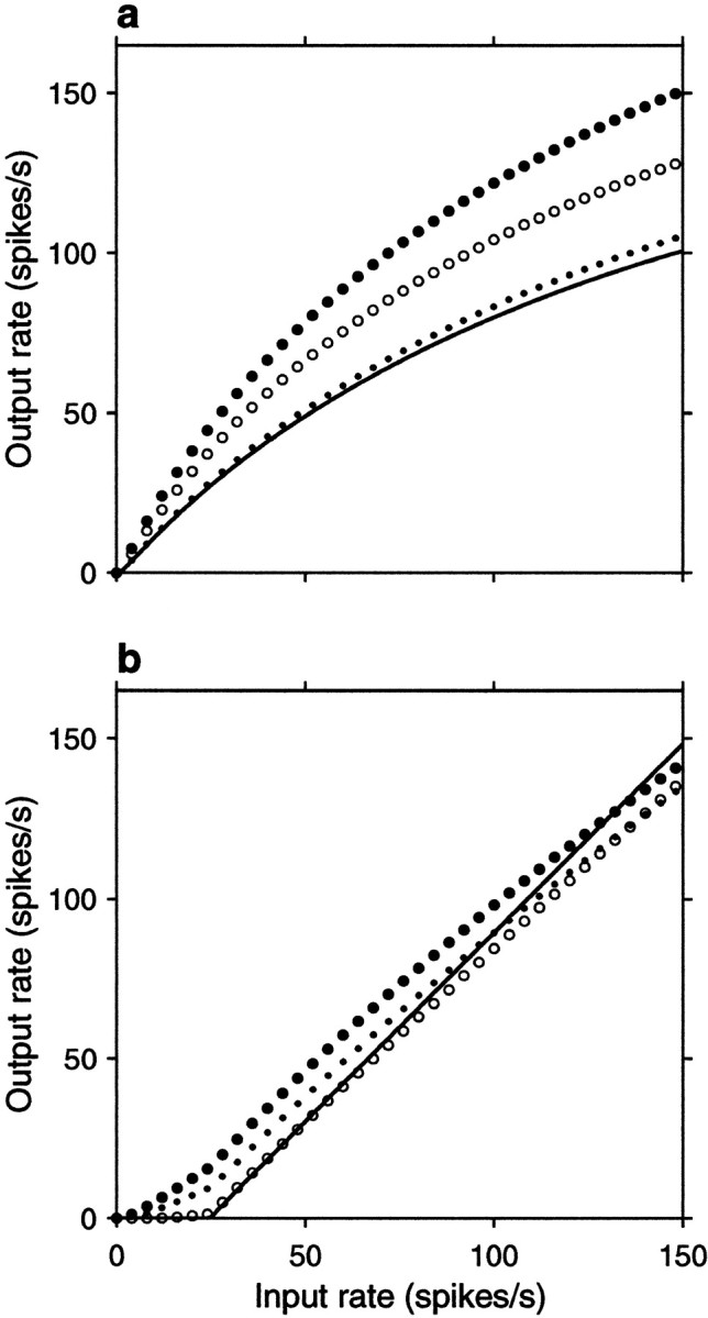
Analytic results from the random walk model. Output firing rate rout is plotted as a function of input rate rE for different parameter values and correlations. To obtain these curves, first, μ and ς were computed from Equations 13 and 19, then Equations 6 and 7 were used. In all plots, the continuous line corresponds to all correlation coefficients equal to zero (uncorrelated inputs),filled circles indicate positive correlations between excitatory pairs only, open circles indicate positive correlations between inhibitory pairs only, and _dots_indicate identical, positive correlations between all pairs.a, Input–output rate curves for a balanced postsynaptic neuron for fixed values of the correlation coefficients. In this case ΔE = 0.5 mV and ΔI/ΔE = 2.35 , which gives βRW = 1 . For the continuous line ρEE = 0, ρII = 0 , and ρEI = 0 . For the filled circles ρEE = 0.0033, ρII = 0 , and ρEI= 0 . For the open circles ρII= 0.0033, ρEE = 0 , and ρEI = 0 . For the _small dots_all three coefficients were equal to 0.0033. b, Input–output rate curve for an unbalanced postsynaptic neuron with ΔE = 0.023 mV and ΔI/ΔE = 0.8 , giving βRW = 0.34 . For these curves all nonzero correlation coefficients were equal to 0.8. Other parameters were, for all plots, as follows: ME = 800, MI = 200, α = 1.7, d = 0.3 mV, Δt = 1 msec, Vθ − Vrest = 20 mV, Vreset − Vrest = 10 mV, and c = 1.7 .
Figure 2a shows the output firing rate as a function of input rate rE for a balanced neuron, for which βRW = 1 (Eq. 13). Here the neuron is driven exclusively by the fluctuations of its inputs, and a fixed amount of net correlation has a multiplicative effect on the firing rate curve, as expected from Equation 19. Figure 2b shows similar curves for a case in which βRW = 0.34 ; for these curves the ratio ΔI/ΔE was modified to obtain an unbalanced neuron that on average received more excitation than inhibition. The input–output rate curve obtained with independent inputs recovers the threshold-linear function typically used in modeling work (Hertz et al., 1991; Abbott, 1994; Koch, 1999). In this case correlations no longer have a multiplicative effect on the routversus rE curve, and the fractional change in output rate caused by a given amount of correlation is much smaller than for a balanced neuron. However, a net excess of excitatory correlations still increases the output rate significantly, especially around threshold (Kenyon et al., 1990; Bernander et al., 1991). This is the point around which the neuron is driven almost exclusively by fluctuations (Bell et al., 1995).
According to this simple stochastic model, the synaptic input that drives a postsynaptic neuron may be thought of as having two components, a mean component, which depends on the net balance between excitation and inhibition, plus another component that represents the fluctuations around the mean, and both components may drive the recipient neuron to fire. The fluctuations depend strongly on the correlations between input spike trains, so it is through their effect on the fluctuations that input correlations may greatly enhance the resulting output firing rate. Such fluctuations may be the main driving force around threshold. The next section explores the validity of these conclusions using more realistic model neurons and computer simulations.
Simulations of a conductance-based integrate-and-fire neuron
Results in this section are based on simulations of an integrate-and-fire neuron model receiving 160 excitatory and 40 inhibitory inputs with Poisson statistics at given mean rates. The amplitudes of the synaptic conductances were varied so that balanced and unbalanced situations could be studied and compared to the predictions from the stochastic model and to Figure 2.
In the random walk model discussed above, input correlations were synonymous with synchrony, because they referred exclusively to the chances of two input spikes arriving in the same time slice Δt . We will show that the results apply to correlations in a wider sense, that is, to situations in which the probability of firing of one input is not independent of the probabilities of the rest of the inputs. We will consider two ways of generating correlated activity, through the equivalent of shared connections and through oscillations in the instantaneous firing rate of the inputs.
Description of the model and parameters
The conductance-based integrate-and-fire model we use is similar to the one described by Troyer and Miller (1997)(Knight, 1972; Tuckwell, 1988;Shadlen and Newsome, 1998; Koch, 1999). The main difference is that we included a mechanism that reproduces the spike rate adaptation typical of most excitatory cortical neurons (McCormick et al., 1985). Subthreshold currents are included, but currents that generate spikes are not. The membrane voltage V(t) changes in time according to the differential equation:
| τm gLdVdt=−gL(V−EL)−ISRA−IAMPA−IGABA+IAPP, | Equation 21 |
|---|
where the first term on the right corresponds to a leak current, and EL is the resting potential. Here we have written the membrane capacitance Cm as τm/Rm, where τm is the membrane time constant and Rm is the input resistance of the neuron, which is equal to the inverse of the leak conductance gL. The I terms stand for specific types of current flowing through the membrane: IAPP corresponds to externally applied (injected) current, and the rest consist of a time-varying conductance g times a driving force, such that:
| ISRA=gSRA(V−EK)IAMPA=gAMPA(V−EAMPA)IGABA=gGABA(V−ECl). | Equation 22 |
|---|
ISRA represents a spike-triggered potassium current that produces adaptation in firing frequency, which is characteristic of most excitatory neurons in the cortex (McCormick et al., 1985). IAMPAand IGABA are the currents produced by fast excitatory and fast inhibitory synapses, respectively. A single isopotential compartment is considered (no spatial variations in V ). The above equations determine the subthreshold behavior of the neuron; whenever V exceeds the threshold Vθ, an output action potential is produced and the neuron enters a refractory period. In practice, when V increases beyond threshold, a spike reaching 0 mV is pasted onto the voltage trace and V is clamped to the value Vreset for a time τrefrac, after which it continues to evolve according to Equation 21.
The conductance changes underlying spike rate adaptation are implemented as follows. Whenever V exceeds Vθ and a postsynaptic spike is elicited, the potassium conductance increases instantaneously by an amount ΔgSRA. The flow of potassium ions tends to hyperpolarize the cell and slows down the firing. The change in conductance decays exponentially toward zero with a time constant τSRA,
| ΔgSRA(t−t0)=g¯SRAexp−t−t0τSRA,t>t0. | Equation 23 |
|---|
Here t0 corresponds to the time at which the output spike was produced, and ΔgSRA is zero for all t < t0. Each subsequent output spike adds an identical conductance change at the corresponding point in time, so the total potassium conductance at any time can be written as the sum of all changes:
| gSRA(t)=∑j ΔgSRA(t−tj), | Equation 24 |
|---|
where tj is the time of output spike j , and the index runs over all output spikes.
The intrinsic model parameters, those independent of synaptic input, were tuned to approximate the neurophysiological measurements ofMcCormick et al. (1985, their Fig. 1_C,D_; see also Troyer and Miller, 1997). The following values are used: EL = −74 mV, EK = −80 mV, Vθ = −54 mV, Vreset = −60 mV, τm = 20 msec, τrefrac = 1.72 msec, τSRA = 100 msec, andg¯SRA = 0.14 gL. These numbers are constant throughout the paper. Figure3 illustrates the behavior of the model in terms of its responses to IAPP, the injected current. In these simulations the input resistance Rm was set to 40 MΩ (that is, gL = 25 nS), but notice that in the rest of the paper, where IAPP = 0 , this parameter is eliminated by expressing all conductances as fractions of gL. Figure 3a shows the firing evoked by a stepwise change in IAPP and illustrates the increase in the interspike intervals that results from the spike rate adaptation current. Instantaneous firing frequency is plotted in Figure3b as a function of applied current. For the curve with circles, frequency was computed as the inverse of the first interspike interval, with 1 sec of zero current between simulated injections; thus the graph corresponds to the unadapted state. For the curve with triangles, frequency was computed as the inverse of the last interspike interval obtained after 1 sec of current injection, at which point firing frequency had adapted fully, reaching a steady state. Again, between current pulses there was a 1 sec intermission. Figure3c plots the lengths of consecutive interspike intervals evoked by different amounts of injected current. The curves rise, reflecting the gradual lengthening of the intervals between output action potentials. ISRA reduces the steady state firing rate to approximately half of the initial, unadapted rate.
Fig. 3.
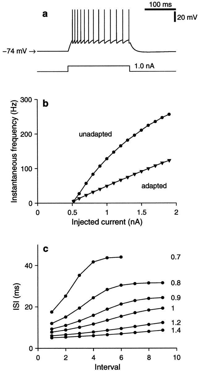
Responses of the conductance-based integrate-and-fire model to current injection. In these simulations, Equation 21 was used with Rm = 40 MΩ ( gL = 25 nS). The applied current IAPP was varied, but no synaptic inputs were included, so IAMPA = IGABA = 0 . Other model parameters as specified after Equation 21.a, The bottom trace shows the time course of a step change in injected current from 0 to 1 nA. The top trace shows the membrane potential of the model. A spike train is elicited by the depolarizing current. The interspike intervals lengthen because of the spike rate adaptation current, ISRA. When the current pulse turns off, the voltage falls below rest (−74 mV) to a minimum of −75.7 mV, later recovering. b, Instantaneous firing frequency as a function of injected current. For the curve with_circles_ (unadapted), instantaneous frequency is equal to the inverse of the first interspike interval elicited by a current pulse; for the curve with_triangles_ (adapted), instantaneous frequency is equal to the inverse of the last interspike interval evoked after 1 sec of current injection. Membrane potential was allowed to relax to rest before all step pulses. c, Lengths of consecutive interspike intervals evoked by step current pulses. These curves reveal the timecourse of adaptation. Each one corresponds to a different current intensity, as is indicated to the right, in nanoamperes. Compare to Figure 1 of McCormick et al. (1985).
Expressions similar to Equation 24 are used to model the conductance changes caused by excitatory synaptic inputs. When an excitatory spike arrives, gAMPA increases by ΔgAMPA. This increase is fast, so a single exponential describing the subsequent decay is sufficient in this case too,
| ΔgAMPA(t−t0)=g¯AMPAexp−t−t0τAMPA,t>t0. | Equation 25 |
|---|
Now t0 corresponds to the time at which the excitatory input arrived, and the transient increase in gAMPA falls off with a time constant τAMPA. Subsequent input spikes add identical conductance changes, so that:
| gAMPA(t)=∑j ΔgAMPA(t−tj). | Equation 26 |
|---|
Now tj is the time of input spike j , and the index runs over all excitatory input spikes. Inhibitory spikes increase the GABA conductance. The rise in gGABA after an inhibitory spike is somewhat slow, so the timecourse of ΔgGABA is better described by the difference of two exponentials,
| ΔgGABA(t−t0)= | Equation 27 |
|---|
g¯GABAD exp−t−t0τGABA(1)−exp−t−t0τGABA(2),t>t0.
Here the D factor is a normalization term that guarantees that the maximum of ΔgGABA is equal to g¯GABA. The two time constants τGABA(1) and τGABA(2) determine the characteristic rise and fall times, as well as D . In this case, t0 corresponds to the time at which the inhibitory input spike arrived, and the total GABA conductance is the sum of the effects of all inhibitory spikes,
| gGABA(t)=∑j ΔgGABA(t−tj). | Equation 28 |
|---|
Additional simulations were performed to explore whether a second, slower inhibitory conductance would affect the results. In these runs the additional conductance followed the same dynamics just described but had a decay time constant of 150 msec. This slow component did not alter the results in any significant way (data not shown) and is not discussed further.
This model neuron does not include any intrinsic sources of noise. In fact, the synapses themselves do not contribute any noise either, because all excitatory or inhibitory spikes cause the same conductance change (the effect of synaptic and intrinsic variability is explored in a separate section below). This allows us to study the impact of input variability in isolation from other noise sources. The model neuron is driven by ME excitatory and MI inhibitory inputs, and each input provides an individual spike train. The mean spike rates are the same for all excitatory and inhibitory inputs; these are rEand rI, respectively. In all simulations, we assume that these rates are proportional, so that rI = αrE, with α being the constant of proportionality. These rates are constant, except when an explicit time dependence is indicated.
The balance of the neuron, β, refers to the ratio between the mean amount of inhibition and excitation that it receives. We measure it asTroyer and Miller (1997) did. This quantity depends on the relative numbers of excitatory and inhibitory inputs, the relative magnitudes of their firing rates, and the relative impacts of excitatory and inhibitory spikes on the postsynaptic voltage. To compute the latter, one should take into account the total changes in conductance integrated over time and the driving forces, so that:
| β≡αMIME GIGE, | Equation 29 |
|---|
where
| GE=‖Vθ−EAMPA‖∫0∞ dtΔgAMPA(t)GI=‖Vθ−ECl‖∫0∞ dtΔgGABA(t). | Equation 30 |
|---|
When β = 1 , there is no mean drift in voltage caused by synaptic inputs; we refer to this as the balanced condition. When β is different from 1 the neuron is unbalanced. Notice, however, that in the literature a balanced neuron is often one that receives some amount of inhibition (β > 0) , as opposed to an unbalanced one which receives only excitation (β = 0) . It seems more appropriate to use the term balanced when excitation and inhibition are truly equilibrated, so in this paper we apply it when β = 1 .
The results shown below are based on simulations that included ME = 160 excitatory and MI = 40 inhibitory inputs. In addition, separate simulations confirmed that the results still hold when the numbers of inputs are increased (data not shown). In these runs the ratio MI/ME was kept constant, and maximal conductance changes were modified accordingly, so that the balance and gain of the neuron remained approximately the same as with the standard numbers of neurons. For the rest of the parameters, the following values are used: α = 1.7, EAMPA = 0 mV, ECl = −61 mV, τAMPA = 5 msec, τGABA(1) = 5.6 msec, and τGABA(2) = 0.285 msec. These numbers are the same in all simulations. For the amplitudes of the conductance changes, two sets of values are considered. In the balanced condition we use g¯AMPA = 0.0806 gL, and g¯GABA = 1.1143 gL, which gives β = 1 . With these parameters, a single excitatory spike yields a maximum depolarization of 0.7 mV at threshold, and a single inhibitory spike yields a maximum hyperpolarization of −1.4 mV at threshold. In the unbalanced condition we use g¯AMPA = 0.0222 gL, and g¯GABA = 0.1382 gL, which gives β = 0.45 . In this case a single excitatory spike yields a maximum depolarization of 0.2 mV at threshold, and a single inhibitory spike yields a maximum hyperpolarization of −0.2 mV at threshold. Having fixed the ratio GI/GE, the maximal conductances were scaled so that, for all conditions tested, the output firing rate rout was close to 75 spikes/sec when the input firing rate rE was set to 100 spikes/sec. This was to allow the neuron to fire at a rate similar to that of any of its inputs (Shadlen and Newsome 1995,1998). Notice that, by expressing the maximal unitary conductances in units of gL, this parameter can be factored out of Equation 21, as long as IAPP= 0 , which is the case for the rest of the paper. Equation 21 was integrated numerically using a fixed time step of 0.05 msec.
Calculation of cross-correlation histograms
In the simulations, a number of excitatory and inhibitory inputs drive a conductance-based integrate-and-fire neuron. We used two methods to generate temporal dependencies between inputs, common drive and temporal comodulations in rate (Brody, 1999). In both cases we computed cross-correlation histograms (Perkel et al., 1967; Fetz et al., 1991; Nelson et al., 1992; Brody, 1999) to visualize the resulting dependencies between pairs of input spike trains. For this, we recorded the firing times of two of the inputs, a and b , for a period of time of length Tmax. Simulation parameters did not change during this time, so the firing statistics of a and b were the same throughout. We use the notation Sa(t) = Σj δ (t − tja) to indicate the spike train of input a , where δ is the Dirac delta function, and tja is the time at which input a fired spike j . The cross-correlation histogram evaluated at time lag τ can be written as:
| Cab(τ)=1C¯ab ∫−Δτ/2Δτ/2 dt′ ∫0Tmax dtSa(t)Sb(t+τ+t′). | Equation 31 |
|---|
The result from the integrals is the number of spikes in the data record that were fired by input b between τ − Δτ and τ + Δτ milliseconds after input a fired; a negative τ corresponds to spikes from b fired before a spike from a . The integral over t′ simply corresponds to the binning associated with the histogram, which has a bin width Δτ . The cross-correlation is normalized by C¯ab, which is the value of the integrals expected for two independent Poisson processes with the same, constant mean rates as the inputs. This factor is:
| C¯ab=rarbTmaxΔτ, | Equation 32 |
|---|
where ra and rb are the mean firing rates of the two inputs. With this normalization, two inputs that fire independently of each other should produce Cab(τ) = 1 at all lags. In practice, because of the discrete character of action potentials, cross-correlograms are quite noisy. To obtain smooth cross-correlograms, we used Tmax between 20 and 30 sec and Δτ = 1 msec, and we averaged over several pairs of inputs (80–120) whose spikes were collected simultaneously from the same simulation.
Generating correlations via common drive
To generate correlated spike trains to be used as inputs to the integrate-and-fire neuron, we used a procedure similar to the one used by Shadlen and Newsome (1998) but somewhat simpler, because it takes advantage of the results in Figure 1. For each of the input lines that impinge on the model postsynaptic neuron, there is a random walk variable that generates the spikes of that line. Variable Ni corresponds to input i and behaves exactly as the model in Figure 1c (blue points), having no net drift and producing a spike whenever Niexceeds a threshold. All random walk variables have the same parameters. At each time step, a set of Mpoolindependent Gaussian random samples with zero mean and unit variance are drawn, and each Ni is updated by adding exactly Min of those samples, weighted by an overall gain factor gin. The sum of Gaussian samples acts as the net input to the random walk units. This is implemented through a matrix multiplication:
| Ni(t+Δt)=Ni(t)+gin ∑j=1Mpool wijsj, | Equation 33 |
|---|
where sj is Gaussian sample j and the entries of matrix w can only be 0 or 1, with exactly Min nonzero terms in each row. If the column indices of the nonzero terms in each row of w are chosen randomly, on average, pairs of input units will share a fraction:
of their Gaussian samples (Shadlen and Newsome, 1998). That is, on average, an input unit will share φMin of its Min samples with any other unit. Any measure of correlation or synchrony between output spike trains generated in this way will be a function of φ, where φ = 0 corresponds to independent trains and φ = 1 corresponds to identical trains. The gain factor gin can be set so that spikes are produced at any desired mean rate. This is done by using Equation 9 and noting that the summation term in Equation 33 has a Gaussian distribution with variance equal to ginMpool. Cross-correlograms between spike trains generated in this way were similar to those reported byShadlen and Newsome (1998), and varying φ was equivalent to varying the fraction of shared connections in their network model.
With this method we generated the 160 excitatory and 40 inhibitory inputs that arrived at the integrate-and-fire model neuron. In the simulations, φE refers to the fraction of samples that each excitatory input draws from the common pool, according to Equation 34 and, similarly, φIrefers the fraction of samples that each inhibitory neuron draws from the pool. A value of φI = 0 means that inhibitory spike trains are independent of each other and of all excitatory spike trains and, analogously, φE = 0 means that excitatory spike trains are all independent. Simultaneous nonzero values for φE and φI correspond to excitatory and inhibitory neurons sharing the same common pool of Gaussian samples, thus being correlated between themselves and across each other's type as well. Notice that these correlated spike trains have a CVISI of approximately one independently of the fraction of shared samples. This is because these neurons are always random walkers drawing their steps from Gaussian distributions with zero mean, as illustrated in Figure 1.
Impact of correlations generated by common drive
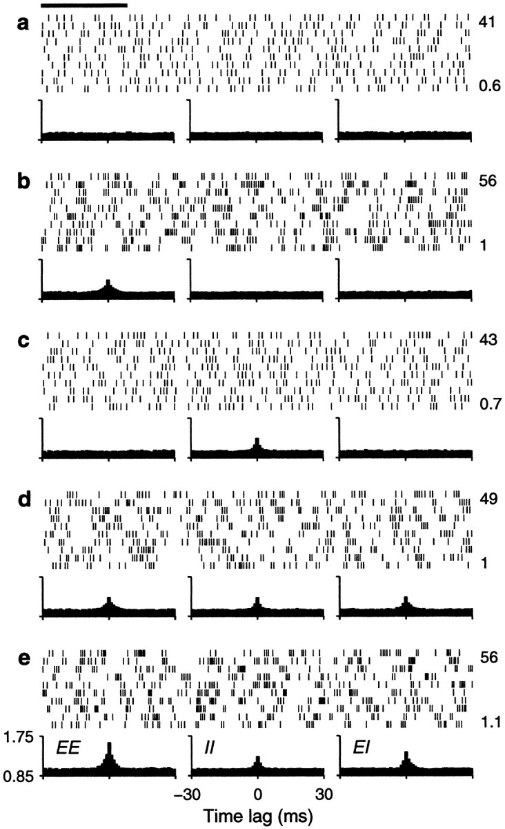
We tested how the output firing rate changed as a function of the fractions of common drive φE and φI. Figure 4shows examples of the output spike trains produced by the balanced integrate-and-fire model. In each panel, the plots below the spike rasters are examples of cross-correlation histograms (Perkel et al., 1967; Brody, 1999) between pairs of input spike trains. The height of the cross-correlation at time lag τ indicates the probability of recording a spike from one neuron between τ − Δτ and τ + Δτ milliseconds after (or before, for negative τ) a spike from another neuron. These histograms have been normalized so that 1 represents the probability expected based on the mean firing rates when the two neurons are independent and follow Poisson statistics. When pairs of input neurons share some of the Gaussian samples, they become correlated—the chances of recording a spike from one neuron are higher around the times when the other neuron has fired. The peaked cross-correlograms shown in the figure were obtained with φ = 0.1 , which is roughly comparable with the measured probability that two nearby pyramidal neurons are connected (Braitenberg and Schüz, 1997). Larger peaks, reflecting stronger synchronization, are common in correlograms constructed from experimental data (Fetz et al., 1991;Nelson et al., 1992).
Fig. 4.
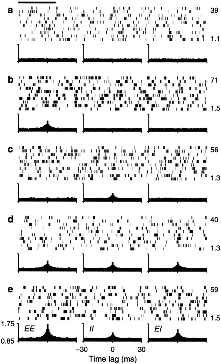
Sample output spike trains from a balanced (β = 1) model neuron for various possible correlation patterns generated by common drive. In each panel, the spike raster shows a 10-sec-long spike train from the output neuron. The full train is shown subdivided into 10 segments of 1 sec duration; each row of the raster corresponds to one segment. The three plots below each raster are cross-correlation histograms between inputs. The ones on the left correspond to excitatory–excitatory (EE) pairs, the ones in the middle correspond to inhibitory–inhibitory (II) pairs, and the ones on the right correspond to excitatory–inhibitory_(EI)_ pairs. Input statistics were constant for each one of the panels. The numbers to the right of the rasters indicate the mean output firing rate (top) and the coefficient of variation of the interspike interval distribution, CVISI_(bottom)_. In all cases, the output neuron was driven by 160 excitatory and 40 inhibitory inputs firing at rates rE = 40 and rI = αrE spikes/sec.a, All inputs were uncorrelated; φE= 0, φI = 0 . b, Only excitatory inputs were correlated; φE = 0.1, φI = 0 . c, Only inhibitory inputs were correlated; φE = 0, φI= 0.1 . d, All inputs were equally correlated; φE = 0.1, φI = 0.1 .e, All inputs were correlated, but excitatory–excitatory pairs were most correlated; φE = 0.2, φI = 0.1 . Calibration: 200 msec. Other parameters as indicated for the balanced condition.
In Figure 4, three histograms are shown below each spike raster. They show the mean correlation between excitatory–excitatory (EE), inhibitory–inhibitory (II), and excitatory–inhibitory (EI) input pairs that drove the output neuron under each condition. These statistical dependencies did not change during the periods in which the shown output spikes were generated. Figure 4a shows a spike train evoked by uncorrelated inputs whose cross-correlations are, consequently, flat. In Figure 4b, only excitatory neurons are correlated, which is evidenced by the peak in the corresponding EE cross-correlation. The small φE of 0.1 that was used makes the output rate increase by ∼60%. As shown in Figure4c, correlations between inhibitory neurons also increase the rate, but the effect is less strong. Correlations in excitatory inputs make a bigger difference because of the parameters chosen. As can be seen from Equations 19 and 20, excitatory or inhibitory inputs may have the largest weight in determining ς2, depending on these choices. With the parameters used in Figure 4, when all neurons are equally correlated the increase in rate practically disappears, as illustrated in Figure 4d. However, Figure4e shows that a large increase in output rate is again seen when all neurons are correlated but excitatory–excitatory pairs are most strongly correlated. Thus, as expected from Equation 19 or 20, it is the balance between the three correlation terms that determines the final contribution of the fluctuations to the output firing rate.
The examples in Figure 4 also show that input correlations can increase the variability of the output neuron. This is most obvious in Figure 4,b and e, which has CVISIvalues of 1.5, much larger than the 1.1 obtained with uncorrelated inputs. In these cases correlations tend to produce more bursts of spikes. With correlations present only between inhibitory neurons (Fig.4c) or when all neurons are equally correlated (Fig.4d), the CVISI still increases slightly, to 1.3, although in the latter case the output rate does not change. Thus, correlations in the input generated through common drive may lead to an increase in output firing rate but, in general, also produce more irregular firing.
Figure 5 expands these results by varying systematically either the input rates or the correlations. Figure5a shows the output firing rate as a function of input rate for uncorrelated inputs, excitatory–excitatory correlations only, inhibitory–inhibitory correlations only, and all possible pairs equally correlated. Figure 5a should be compared with Figure2a, which depicts the analogous curves expected from the random walk model. To compare the two sets of results, parameter ΔE was scaled so that the analytic curves with uncorrelated inputs would have approximately the same gain as in the simulation, and the value of 0.004 used in Figure 2a for the correlation coefficients was chosen to match the effects seen in Figure5a. The curves obtained with the conductance-based model are in excellent agreement with the analytical predictions from the random walk equations, in spite of the numerous details that distinguish the two models. Figure 5c shows how the output rate changes as a function of correlation strength for a fixed input rate, rE = 40 spikes/sec. As expected, higher correlations have stronger effects. For a balanced neuron, even a weak correlation between its excitatory inputs may have a large impact on the output; a fraction of shared samples of ∼0.15 (φE = 0.15) is enough to double the output firing rate.
Fig. 5.

Effect of input correlations generated by common drive on the firing rate and variability of the same balanced (β = 1) model neuron used in Figure 4. For each data point, the output spike train was recorded for 30–90 sec of simulation time, and the mean rate and coefficient of variation were computed from this segment. a, Mean output firing rate rout as a function of input rate rE, for four conditions. The continuous line indicates uncorrelated inputs (φE = 0, φI = 0) , filled circles indicate correlations between excitatory inputs only (φE = 0.1, φI = 0) ,open circles indicate correlations among inhibitory inputs only (φE = 0, φI = 0.1) , and dots indicate all pairs equally correlated (φE = 0.1, φI = 0.1) .b, CVISI of the output spike trains as a function of input rate, computed from the same simulations as in_a_; symbols have identical meaning. The_dashed line_ marks a CVISI of 1, expected from a Poisson process. c, Mean output firing rate rout as a function of correlation strength, for a fixed input rate rE = 40 spikes/sec.Filled circles correspond to correlations between excitatory neurons only (φE varies along the x axis and φI = 0) , _open circles_correspond to correlations between inhibitory neurons only (φE = 0 and φIvaries along the x axis), and dots correspond to all pairs equally correlated (φE and φI vary identically along the x axis). d, CVISI of the output spike trains as a function of correlation strength, computed from the same simulations as in c; symbols have identical meaning. Other parameters as indicated for the balanced condition.
Figure 5, b and d, shows that correlations also increase the variability of the output neuron, as measured by the CVISI. For the balanced condition, the increase is larger at low output rates. Notice that, even in the absence of correlations, CVISI increases with increasing input rate, as shown by the continuous line in Figure 5b . With high input rates or with modest correlations, output variability may easily increase past a CVISI of ≥1. This constitutes a major difference between the random walk description and the conductance-based model. When the changes in membrane potential are described by a random walk, the neuron is memoryless: what happens in one Δt has no influence on what happens in the next and, similarly, one interspike interval has no relation to the next. This leads to values of CVISI ≤1, if there is some net drift. Conductance changes, however, are not instantaneous so, for instance, several synchronous excitatory spikes may produce a burst of output spikes instead of the single spike expected from the random walk model. Thus, conductances allow much greater variability in the output spike train than instantaneous “adding” of spikes.
It is well known that refractoriness also affects spike train variability (Koch, 1999). The simulations in Figures 4and 5 were obtained with synaptic time constants of ∼5 msec and a refractory period of 1.72 msec. We also ran simulations in which all synaptic time constants were divided by a factor of 2.5, and the maximal conductances were increased to produce the same gain and balance. This made the refractory period much larger relative to the timescale of unitary changes in postsynaptic conductance. The only difference observed in these simulations was that all CVISI values were smaller than those of Figures4 and 5 by ∼0.2; otherwise, correlations had the same effects on rate and caused the same relative increases in CVISI.
The simulation results presented so far were obtained with a balanced neuron. However, it is not certain whether values of β as large as 1 are within the physiologically plausible range (Berman et al., 1991; Douglas and Martin, 1998; Stevens and Zador, 1998). Therefore, it was important to investigate whether the results were also valid with an unbalanced neuron with low β. The corresponding simulation results are shown in Figures 6 and 7, in the same format as Figures 4 and 5 but for an integrate-and-fire model with β = 0.45 . In viewing Figure 6 it is important to recall that the plots below the rasters are cross-correlation histograms between pairs of input spike trains. These histograms reveal the statistical dependencies of excitatory and inhibitory inputs, which were constant in each one of the panels.
Fig. 6.
Sample output spike trains from an unbalanced (β = 0.45) model neuron for various possible correlation patterns generated by common drive. Same format and correlation values as in Figure 4, except that rE = 60 spikes/sec. Other parameters as indicated for an unbalanced neuron.
Fig. 7.

Effect of input correlations generated by common drive on the firing rate and variability of the same unbalanced (β = 0.45) model neuron used in Figure 6. Same format and input parameters as in Figure 5, except that, in c and d , rE = 60 spikes/sec. Parameters of the postsynaptic neuron as indicated for the unbalanced condition.
The spike rasters in Figure 6 show that the same amount of correlation now produces, overall, a small enhancement in rate that is not multiplicative. Nevertheless, a fraction φE = 0.1 still raises the output rate by ∼10 spikes/sec when the input rate is <80 spikes/sec or so. On the other hand, correlations still cause a large increase in CVISI. Note, in particular, that the increase is seen even when the three correlation terms are identical. This is because the relative values of their coefficients in Equation 19 do not produce a full cancellation. Here, however, the neuron is much less variable to begin with (that is, with uncorrelated inputs), and the CVISI is almost flat as a function of input rate. Thus, as shown in Figure7b, in the presence of weak correlations CVISI stays around or <1 at all input rates considered. As in the balanced condition, additional simulations were also run using faster synaptic timescales, but this made practically no difference on the results; refractoriness played a minor role in this case.
Figure 7a shows the impact of input correlations on the input–output firing rate curve of an unbalanced neuron. Note, in particular, that correlations effectively decrease the threshold (Kenyon et al., 1990; Bernander et al., 1991; Bell et al., 1995). These curves should be compared with those in Figure 2b, which correspond to the random walk model in the presence of a large drift, or net excitatory drive. The match between the two sets of curves is not perfect, but the shape of the rate curve and the changes caused by the presence of input correlations are well described by the theoretical expressions. Thus, although parameter values used in Figure 2, a and_b_, were adjusted to optimize overall agreement between the two models, the predictions of the stochastic model, particularly the differences between balanced and unbalanced regimes, are remarkably accurate, considering its simplicity.
Impact of correlations generated by oscillations
The firing probabilities of two neurons may fluctuate in time around some fixed average. If such temporal fluctuations tend to occur together, the two neurons will be correlated; the probability of one of them firing will be higher when the other one also fires, because this will reflect an upward increase in the underlying firing rates. We investigated whether inputs that become correlated in this way produce effects similar to the ones observed through common drive. For this, we modeled input firing rates as periodic functions of time, such that:
| rE(t)=AE(1+εEsin(2πft)) | Equation 35 |
|---|
| rI(t)=αAE(1+εIsin(2πft)), | Equation 36 |
|---|
where f is the frequency of the oscillations, and the mean firing rates are AE for excitatory and αAE for inhibitory neurons, respectively. The probability that a particular excitatory neuron fires a spike at time t is then rE(t)Δt , and similarly for inhibitory inputs. Parameters εE and εI control the modulation amplitude around the mean. When the rates vary according to the above equations, any measure of correlation is a function of these two numbers. For example, εE = 0 implies that excitatory neurons are uncorrelated. In the simulations these parameters were always between 0 and 1.
Figure 8 shows sample spike trains from the balanced integrate-and-fire neuron when the input rates vary periodically at a frequency f = 40 Hz. As before, the plots below the voltage traces are cross-correlation histograms, which show the statistical dependencies between inputs in each condition. The different panels correspond to different values of εE and εI. For comparison, Figure 8a shows a response to uncorrelated inputs; this case corresponds to all cross-correlation histograms being flat. When only rE fluctuates in time, as shown in Figure 8b, excitatory inputs become correlated, their cross-correlation histogram reflects the periodicity of the underlying rates, and the output neuron fires more strongly. Based on the results of previous sections, this is precisely what is expected when net excitatory correlations are present. In addition, the output neuron fires in bursts, reflecting the underlying input oscillations. Other possible correlation patterns also modify the output firing rate as predicted: co-fluctuations between inhibitory neurons also enhance the output rate, and when all possible pairs are equally correlated the enhancement practically disappears. Figure 8e shows a variant of this latter case in which a phase difference exists between excitatory and inhibitory rates (for a similar situation in real neural circuits, see Skaggs et al., 1996; Tsodyks et al., 1997). For this plot, εE and εI were both equal to 0.6, but we used a cosine instead of a sine in Equation 36. This introduced a time delay of 6.25 msec between the peaks of rE(t) and rI(t) , which is reflected in the cross-correlogram between excitatory and inhibitory neurons (Fig.8e, EI ). In this situation the output rate is greatly enhanced; it is almost twice that obtained with uncorrelated inputs. Here all input pairs are correlated, but at slightly different times. This produces the greatest excitation at a time when inhibition is not at its peak. This result demonstrates that the timing of correlations also plays a crucial role in determining the output firing rate.
Fig. 8.

Sample output spike trains from a balanced (β = 1) model neuron driven by inputs whose rates oscillate in time. In each panel, the 500 msec voltage trace shows the response of the model neuron. The three plots below each raster are cross-correlation histograms between inputs. The ones on the_left_ correspond to excitatory–excitatory (EE) pairs, the ones in the middle correspond to inhibitory–inhibitory (II) pairs, and the ones on the_right_ correspond to excitatory–inhibitory (EI) pairs. Input statistics were constant for each one of the panels. The_numbers_ to the right of the rasters indicate the mean output firing rate from the traces shown. In all cases, the output neuron was driven by 160 excitatory and 40 inhibitory inputs firing at rates given by Equations 35 and 36 with AE = 40 spikes/sec and f = 40 Hz. a, All input rates were constant; εE = 0, εI = 0 . b, Only excitatory inputs were oscillating; εE = 0.6, εI = 0 . c, Only inhibitory inputs were oscillating; εE = 0, εI = 0.6 . d, All inputs were oscillating with the same frequency and phase; εE = 0.6, εI = 0.6 .e, All inputs were oscillating at the same frequency, but a cosine instead of a sine was used in Equation 36 for rI(t) . A phase difference between excitatory and inhibitory rates is apparent in the EI cross-correlation. For this plot εE = 0.6 and εI= 0.6 . Calibration: 100 msec. Other parameters as indicated for the balanced condition.
Figure 9 expands these results by varying the input rates and correlations throughout a range. This figure has the same format as Figure 5, except that εEand εI vary along the x axes in Figure 9, c and d, because they determine the correlation strengths in this case. The symbols also have the same meanings as in Figure 5, except that nonzero values of φE and φI now correspond to nonzero values of εE and εI. The curves in Figure 9_a_obtained with the conductance-based model are again in good agreement with the analytical results from the random walk model. The major difference is the greater effect that inhibitory oscillations have on output rate. This occurs because, with oscillatory rates, the variance in the number of spikes produced by each input per Δt depends more strongly on the firing rate than what was assumed before (the difference is the step between Equations 18 and 19: with oscillatory rates, different expressions for sE2 and sI2should be used, and this results in different coefficients for the ρ terms). Inhibitory correlations are stronger in this case because inhibitory inputs fire faster than excitatory ones.
Fig. 9.

Effects of correlations generated by oscillating input rates on the firing rate and variability of the same balanced (β = 1) model neuron used in Figure 8. For each data point, the output spike train was recorded for 30–90 sec of simulation time, and the mean rate and coefficient of variation were computed from this segment. a, Mean output firing rate rout as a function of mean input rate AE, for four conditions. The continuous line indicates uncorrelated inputs (εE = 0, εI = 0) , filled circles indicate oscillating excitatory inputs (εE = 0.6, εI = 0) , open circles indicate oscillating inhibitory inputs (εE = 0, εI = 0.6) , and dots indicate all input rates oscillating identically (εE = 0.6, εI = 0.6) . b, CVISI of the output spike trains as a function of mean input rate, computed from the same simulations as in_a_; symbols have identical meaning. The_dashed line_ marks a CVISI of 1.c, Mean output firing rate routas a function of correlation strength for a fixed mean input rate AE = 40 spikes/sec. Filled circles correspond to oscillating excitatory inputs (εE varies along the x axis and εI = 0) , open circles_correspond to oscillating inhibitory inputs (εE = 0 and εIvaries along the x axis), and dots correspond to all inputs oscillating with the same frequency and phase (εE and εI vary identically along the x axis). d, CVISI of the output spike trains as a function of correlation strength, computed from the same simulations as in_c; symbols have identical meaning. Other parameters as indicated for the balanced condition.
As shown in Figure 9c, larger correlations still produce larger increases in rate. Overall, the effects on output rate of correlations induced by temporal co-fluctuations in firing probability are similar to those produced by common drive to the inputs. On the other hand, as shown in Figure 9, b and d, the variability of the output spike trains tends to decrease when input rates oscillate, as indicated by the CVISI. This is not surprising because, in this case, input firing is more regular, and the output spikes tend to follow the periodic increases in excitation.
Figures 10 and11 show the corresponding results for the unbalanced postsynaptic neuron with β = 0.45 . As was shown above, the unbalanced neuron is less sensitive to correlations than the balanced neuron. However, as seen in Figures 10and 11a, the temporal modulation of excitatory input rates using εE = 0.6 still raises the output rate by ∼10 spikes/sec when the mean input rate is <80 spikes/sec approximately, and the effect still increases monotonically as correlations become stronger, as indicated in Figure 11c. Oscillations, however, seem to be less effective in driving the target neuron when it is below threshold, as can be observed by comparing Figures 11a and 7a (insets). It should also be borne in mind that higher rates will be evoked whenever there is a phase difference between excitatory and inhibitory inputs, as illustrated in Figure 8e.
Fig. 10.

Sample output spike trains from an unbalanced (β = 0.45) model neuron driven by inputs whose rates oscillate in time. Same format and correlation values as in Figure 8, except that AE = 60 spikes/sec. Other parameters as indicated for the unbalanced neuron.
Fig. 11.

Effects of correlations generated by oscillating input rates on the firing rate and variability of the same unbalanced (β = 0.45) model neuron used in Figure 10. Same format and input parameters as in Figure 9, except that, in_c_ and d, rE = 60 spikes/sec. Parameters of the postsynaptic neuron as indicated for the unbalanced condition.
In summary, as far as output firing rate goes, the presence of input correlations has similar effects regardless of the mechanism by which those correlations are generated, and such effects are well described by the theoretical model developed above. A comparison between Figures2a, 5a, and 9a shows that this is true for a balanced model neuron, and a comparison between Figures2b, 7a, and 11a shows that this is also true for an unbalanced neuron. In contrast to the rate, the variability of the interspike intervals is sensitive to the dynamics that give rise to the correlations. Correlations arising from common drive tend to increase the CVISI of the output, whether the postsynaptic neuron is balanced (Figures 5b, d) or not (Figures 7b, d), whereas correlations arising from periodic, temporal co-fluctuations in rate have a weaker tendency to decrease the CVISI when the postsynaptic neuron is balanced (Figures 9b, d), and their effect on an unbalanced neuron may be either upward or downward (Figure11b).
Impact of other factors contributing to input variance
A general implication of the analytic results presented here is that a balanced neuron responds to variance in synaptic input: variance is its driving force. In the stochastic model, variability in the statistics of input spikes provided all the variance, but synapses themselves also behave stochastically, and so do the channels and receptors on the postsynaptic membrane (Calvin and Stevens, 1968). Including synaptic variability corresponds to considering a ΔE that is not constant, but rather comes from a distribution. If the theoretical analysis is correct, unreliable, stochastic synapses that on average produce a change in voltage of a given size should give rise to larger firing rates than perfectly reliable synapses that always produce a depolarization of the same mean size. In this case, failures in synaptic transmission may actually boost the output firing rate, because large but infrequent depolarizations have a better chance of causing a spike than small and frequent ones.
To study this, we allowed synaptic failures in the conductance-based model. In this case, whenever an input spike arrives, the synaptic conductance can do two things, either increase by an amount Δg(t)/PT (as in Eqs. 25 and 27), or remain the same, as if no spike had arrived. The first option corresponds to successful transmission and occurs with probability PT; the second option corresponds to a failure and occurs with probability 1 − PT. With this scheme, the mean conductance change averaged over many input spikes is always the same (and equal to Δg(t) ) regardless of the probability of transmission PT. The case PT = 1 corresponds to zero failures, as was considered in all previous results.
Figure 12 shows how the output rate and CVISI change when synapses are allowed to fail. For this figure, the dynamics described in the previous paragraph were applied to AMPA and GABA conductances, with separate PT values for each. Based on experimental reports (Murthy et al., 1997), we chose PT = 0.15 . Figure 12, a and_b_, corresponds to a balanced postsynaptic neuron, and Figure12, c and d, corresponds to an unbalanced one, with the same sets of parameters used before. For these curves, all inputs were uncorrelated. The curves are in good agreement with the theory: failures increase input variance and, when the neuron is balanced, this produces an increase in gain. In contrast to spike train correlations, inhibitory failures cause larger effects than excitatory ones. This can be understood by calculating the variance of ΔV across time steps. Starting from Equations 2 and 3, we proceed as in the calculation of Equation 18, but assume that the unitary voltage changes ΔE and ΔI have binomial distributions with means 〈ΔE〉 and 〈ΔI〉 . In the absence of correlations, the variance of ΔV is then:
| sE2ME〈ΔE〉2+sI2MI〈ΔI〉2+ | Equation 37 |
|---|
rEΔtME〈ΔE〉2 1−PTEPTE+αMI〈ΔI〉2 1−PTIPTI,
where PTE and PTIare the transmission probabilities for excitatory and inhibitory synapses, respectively. When these are equal to 1, only the first two terms in the expression survive, and the original variance equal to 〈ΔE〉2 ς2 is recovered (this is obtained from Eqs. 3 and 18 with zero correlations and constant ΔE). When the probabilities are <1, contributions from excitatory and inhibitory failures increase the variance. In the balanced condition αMI〈ΔI〉2 is much larger than ME 〈ΔE〉2 (Fig. 2, legend) so, for similar transmission probabilities, the contribution from inhibitory failures is bigger than the contribution from excitatory ones, in agreement with Figure 12a. The effect of failures can also be thought of as an increase in ς2. To see this, first, obtain an effective ς2 by factorizing the quantity 〈Δ_E_〉2 from the above equation; the result is:
| sE2ME+sI2MI 〈ΔI〉2〈ΔI〉2+rEΔtME 1−PTEPTE+αMI 〈ΔI〉2〈ΔE〉2 1−PTIPTI. | Equation 38 |
|---|
Second, compare this to Equation 18, assuming zero correlations. For fixed values of 〈ΔE〉 and 〈ΔI〉 , failures behave as if they changed ς2. This explains why in the results of Figure12a it appears as if failures increased the variance of the spike counts.
Fig. 12.

Effects of synaptic failures on the firing rate and variability of a target model neuron. In all cases inputs were uncorrelated. For every incoming spike, a failure in transmission could occur with probability 1 − PT, in which case no conductance change was elicited. Transmission occurred with probability PT, and in this case a conductance change took place as in previous simulations (Eqs. 25, 27), except that maximal conductances were multiplied by a factor of 1/PT. Continuous lines indicate PT = 1 for all inputs; filled circles indicate PT = 0.15 for excitatory and PT = 1 for inhibitory synapses; open circles indicate PT = 1 for excitatory and PT = 0.15 for inhibitory synapses; and dots indicate PT = 0.15 for both excitatory and inhibitory synapses. For each data point, the output of the postsynaptic neuron was recorded for 30–90 sec of simulation time, and the mean rate and coefficient of variation were computed from this segment. a, Mean output firing rate rout as a function of mean input rate rE for a balanced neuron with β = 1 . b, CVISI of the same target neuron used in a, as a function of mean input rate. c, d, as in a and b but for an unbalanced neuron with β = 0.45 . Inset amplifies the region around threshold. Other parameters as indicated for balanced and unbalanced conditions.
In contrast to correlations, synaptic failures always add more variance. This is because excitatory and inhibitory synapses release their neurotransmitters independently of each other, so there is no negative term equivalent to ρEI. The small dots in Figure 12a show that a larger increase in mean output rate is obtained when both excitatory and inhibitory synaptic failures are included, as expected from the two equations above. As shown in Figure 12c, for the unbalanced neuron the increase in rate is much smaller, but still appreciable, especially near threshold. Lowering of firing threshold attributable to increased variance in membrane potential fluctuations has also been observed in more detailed neuronal models (Bernander et al., 1991;Destexhe and Hô, 1999; Hô et al., 2000).
According to this result, an excitatory presynaptic neuron may be more effective, on average, when it makes a synaptic contact of strength 2 S that fails half the time, than when it makes a contact of strengths S that never fails. Thus, synaptic failures and synchronous spikes give rise to similar effects on the postsynaptic membrane. This may seem counterintuitive, but the key is that both increase the variance in synaptic drive, and variance drives the neuron when the mean drive is small in comparison.
The intrinsic variability of the postsynaptic membrane also contributes to the variance of the membrane potential. This means that, in a balanced neuron driven exclusively by fluctuations, intrinsic membrane noise should produce an upward shift in the output versus input firing rate curve. We confirmed this through simulations in which, on each integration time step, independent Gaussian noise with zero mean was added directly to the voltage of the postsynaptic neuron. The output rate of the target neuron indeed increased with added Gaussian noise as expected for balanced and unbalanced conditions and, interestingly, Gaussian noise could also decrease the CVISI in both cases (data not shown; Tiesinga and José, 1999). To observe these effects it was necessary to inject relatively large amounts of noise (we used a SD of 0.17 mV). Experimental findings (Calvin and Stevens, 1968;Mainen and Sejnowski, 1995; Holt et al., 1996) and theoretical arguments (Softky and Koch, 1993) indicate that statistical fluctuations caused by spike-generating mechanisms should be much smaller than those produced by variations in spike arrival times. In agreement with these observations, we found that intrinsic membrane noise had much less impact on firing rate and interspike interval variability than input correlations. The reason for this, from Equations 19 and 20, is that the correlation terms are multiplied by the square of the corresponding numbers of inputs, which are at least in the hundreds. Therefore, even weak correlations may contribute much more than other noise sources to fluctuations in membrane potential.
DISCUSSION
The impact of input correlations on the mean firing rate of a postsynaptic neuron was calculated using a simple stochastic model. The analytical results (Fig. 2) were confirmed through simulations of a conductance-based, integrate-and-fire neuron driven by hundreds of synaptic inputs. In this framework, the process of synaptic integration can be cast as follows. Both the drift, or mean net drive μ—average excitation minus inhibition minus decay caused by leakage—and the fluctuations around this mean may cause a postsynaptic neuron to fire (Troyer and Miller, 1997). Correlations between excitatory neurons or between inhibitory neurons increase the variance ς2 of the fluctuations, whereas correlations between excitatory–inhibitory pairs decrease it. Correlations have their largest impact upon fully balanced neurons (μ ≤ 0), because these are driven exclusively by fluctuations. However, even in unbalanced neurons weak correlations may have a significant impact around firing threshold, because at that point it is usually the case that μ ≈ 0. By weak we mean shared input with φ = 0.1 , which corresponds roughly to the probability that two nearby excitatory cortical neurons are connected (Braitenberg and Schüz, 1997;Shadlen and Newsome, 1998).
The theoretical model did not provide an expression for the variability of the interspike interval distribution of the postsynaptic neuron, but it did bound its coefficient of variation CVISIbetween 0 and 1, depending on which contributed more to the firing of the neuron, μ or ς. When ς = 0 and μ > 0 , a neuron fires regularly, like a clock, and when ς > 0 and μ ≤ 0 , it fires irregularly, like a Geiger counter. These facts are useful in reviewing previous studies regarding neuronal variability.
The spike trains of neurons recorded in awake animals are extremely variable (Burns and Webb, 1976; Dean, 1981; Softky and Koch, 1993; Holt et al., 1996; Stevens and Zador, 1998; Shinomoto et al., 1999), but spike generation mechanisms themselves seem to be highly reliable (Calvin and Stevens, 1968;Mainen and Sejnowski, 1995; Holt et al., 1996). Therefore, although intrinsic properties may still be important (Bell et al., 1995; Troyer and Miller, 1997), the variability of a neuron in an intact microcircuit should come mostly from the variability of its inputs. Softky and Koch (1992, 1993) pointed out that, although the CVISI of typical cortical neurons is close to 1, this number should be much lower for an integrator that adds up many small contributions to fire, especially at high output rates. They found that, in the absence of inhibition, high CVISI values could be obtained either with an unrealistically small (i.e. submillisecond) membrane time constant, or using active dendrites that worked as isolated coincidence detectors (Abeles, 1982, 1991; Softky, 1993;Shadlen and Newsome, 1994). In our integrate-and-fire model, a smaller time constant τm also produced higher CVISI values, but otherwise it did not alter the effects of correlations (time constants down to 1 msec were tested; results not shown). Shadlen and Newsome (1994) later showed that, as in earlier stochastic models (Gerstein and Mandelbrot, 1964; Tuckwell, 1988; Smith, 1992), including incoming inhibitory spikes produces high CVISI values. Their model was nearly balanced. Troyer and Miller (1997) extended these results by carefully tuning an integrate-and-fire neuron to produce a relatively high CVISI while using biologically plausible amounts of inhibition (Bell et al., 1995). Their simulation results fell in the lower half of the range 0.5 to 1 reported bySoftky and Koch (1993). More recently, Stevens and Zador (1998) (see also Destexhe and Paré, 2000) have also suggested, based on experiments in a slice preparation, that input synchrony is required to produce the high variability observed in vivo. This is consistent with the suggestion that stochastic eye movements, which provide a common, correlating signal, are responsible for a large fraction of the variability observed in primary visual neurons (Gur et al., 1997). It also agrees with recent theoretical results (Feng and Brown, 2000), and with simulation studies in which network interactions produce synchronized recurrent input, which also leads to high variability (Usher et al., 1994;Tsodyks and Sejnowski, 1995; Van Vreeswijk and Sompolinsky, 1996).
In the unbalanced condition, we found that weak correlations generated by common drive to the inputs could raise the CVISI from ∼0.6 to 1 (Stevens and Zador, 1998). This could result from correlations between excitatory neurons only or between all inputs (Fig. 7b;Feng and Brown, 2000). We also observed that correlations could raise the CVISI of the conductance-based model well beyond 1 (Figure 5b, d), even in the unbalanced condition (Fig. 7d). This is in marked contrast to our random walk model and to other models based on memoryless processes where, it should be noted, the refractory period (or dead time) may play an important role in limiting the CVISI (Smith, 1992; see alsoTuckwell, 1988; Shadlen and Newsome, 1998; Koch, 1999; Shinomoto et al., 1999).
Earlier studies also explored the relationship between input correlation and output rate. Bernander et al., (1994)and Murthy and Fetz (1994) found that synchrony could increase the firing rate of the target cell but only up to a point, after which the rate tended to decrease. This happened because, on one hand, leakage tends to erase the effect of previous inputs, so these should come close together in time to avoid wasting depolarization. But on the other hand, synaptic inputs that arrive during the refractory period have little or no effect, and to avoid this situation inputs should be somewhat spread out in time. The tradeoff between these two conditions, as well as the degree of correlation between inputs, gives rise to an optimal time window for synaptic integration. However, this scenario is valid when excitation is overwhelmingly larger than inhibition and when the output neuron is firing intensely, such that refractory effects become important. In this unbalanced regime the postsynaptic cell operates at a low gain—in these studies, at least 100 (net) excitatory input spikes were required to produce a single output spike—and firing is much more regular than observed experimentally. Because neurons fire irregularly and appear to operate at high gain (Softky and Koch, 1992, 1993;Shadlen and Newsome, 1994, 1998; Troyer and Miller, 1997), the effects in low gain models may be small within the normal dynamic range of real neurons. In our simulations, the effects of correlations did not vary appreciably with the refractory period.
Softky and Koch (1993) (see also Ritz and Sejnowski, 1997) also noticed that synchronized inputs produced higher output firing rates than independent inputs. They observed this for positive correlations between excitatory pairs. Other studies (Sejnowski, 1976; Kenyon et al., 1990;Bernander et al., 1991; Bell et al., 1995) are also consistent with our finding that an unbalanced neuron should be considerably more sensitive to synchronous excitatory spikes than to uncorrelated ones. In contrast, Shadlen and Newsome (1998) studied the effect of input synchrony and found that even fractions of shared connections among inputs as large as 0.4 did not elicit any change in the statistics of a target neuron. Their model was fully balanced, so the output rate must have been most sensitive to the presence of correlations. However, they chose parameters for which ς2 is given by Equation 20 and, because they used identical correlations among all possible pairs, the three correlation terms cancelled out exactly.
This brings us to the two experimental questions that are crucial to evaluate the impact of correlations. First, what is the actual balance between excitation and inhibition? In our models, inhibition countered excitation through changes in conductance and firing rate, but other factors like synaptic location are also important. Whatever the biophysical implementation, balance is crucial because, according to our models, it determines whether input correlations affect the gain of a neuron either throughout its full dynamic range or mostly at low firing rates. Second, what are the relative magnitudes of the three correlation terms in typical cortical circuits? At the moment, experimental data seem insufficient to determine this. Based on anatomical considerations (White, 1989;Braitenberg and Schüz, 1997) and neurophysiological measurements (Fetz et al., 1991;Nelson et al., 1992; Zohary et al., 1994;Salinas et al., 2000), it seems likely that all terms are different from zero, at least for local microcircuits; but what really needs to be known is the final weighted sum. This final sum might not be constant, neither in time nor across cortical areas. Here we illustrated various possible combinations of the three terms and found that even a small net deviation from zero may have a large impact on output gain and variability. Given such high sensitivity, perhaps the correlation structure between neurons is dynamically modulated. Recent experiments suggest that synchrony may covary with attention (Steinmetz et al., 2000). Furthermore, because the timing of correlations may also enhance their effects (Fig.8e), correlations could also interact with normal plasticity mechanisms that depend on spike timing (Linden, 1999;Sejnowski, 1999; Paulsen and Sejnowski, 2000). Therefore, dynamic changes in correlations could have profound functional implications (Singer and Gray, 1995;Shadlen and Newsome, 1998).
It is interesting that our model neurons may encode the statistical properties of their inputs in different ways, depending on their balance. In a balanced neuron, output firing rate and variability are both sensitive to input rate and to correlations, and the input–output rate curve is nonlinear (Fig. 5a,b). On the other hand, in an unbalanced neuron output rate is only modestly sensitive to input correlations, the input–output rate curve is practically linear, except for the threshold, and variability is sensitive to correlations but much less so to input rate (Fig. 7a,b). The next step is to explore the statistics of spike trains in feedback models and to relate these to the functional properties of cortical circuits (Singer and Gray, 1995; Tsodyks and Sejnowski, 1995; Van Vreeswijk and Sompolinsky, 1996;Shadlen and Newsome, 1998).
Here we derive Equations 6 and 7, which give the firing rate of the stochastic neuron as a function of μ and ς, the mean and SD, respectively, of the net number of excitatory inputs that arrive at the neuron in one Δt . We make use of Equations 1-5.
The methods used to develop the stochastic model are standard in the mathematics and physics literature. The present model is closely related to the Ornstein–Uhlenbeck process, for which a closed-form solution is not known, although asymptotic expansions have been found (Ricciardi, 1977; Smith, 1992;Shinomoto et al., 1999). The major difference is that the Ornstein–Uhlenbeck process includes a term proportional to −V in Equation 1, a true leak, which drives the membrane potential toward rest. The constant decay assumed here and represented by the term d is thus a key simplification. As general references on stochastic processes and on the computation of first passage times the reader may consult, for example, the books byRicciardi (1977), Tuckwell (1989), orRisken (1996); see also Berg (1993) for applications to other problems in biology.
First consider a situation analogous to a purely random walk without drift, for which μ = 0 . Assume that the distribution function P is symmetric, so that P(n) = P(−n) for any n . In this case, the mean number of steps needed to reach a threshold, as a function of N , obeys the relationship:
| ν(N)=1+∫0∞ [ν(N+n)+ν(N−n)]P(n)dn. | Equation 39 |
|---|
This equation is a generalization of the classic random walk in which the magnitude of the step is constant and positive and negative steps are equally probable (Berg, 1993) (see alsoFeynman et al., 1963). In that case the integral corresponds to a sum of only two terms, with P = 1/2 . This expression follows from the fact that, in a single time step, N can go from its present value to either N + n or N − n with equal probabilities, hence the requirement that P be symmetric. From this expression, a differential equation for ν can be derived assuming that n is small relative to N (Berg, 1993). The alternative approach that follows leads to a similar solution but highlights its key properties and limitations more clearly.
Recalling that the integral over all probabilities must be equal to 1, the above expression can be rearranged as:
| 1+∫0∞ [ν(N+n)+ν(N−n)−2ν(N)]P(n)dn=0. | Equation 40 |
|---|
Suppose the solution is a polynomial:
| ν(N)=∑j=0 cjNj, | Equation 41 |
|---|
where the ci are constant coefficients. For the function ν(N) to satisfy Equation 40, the term in brackets must be a function of n only; it cannot depend on N . This condition is satisfied when:
| ν(N)=c0+c1N+c2N2, | Equation 42 |
|---|
and all other terms have cj = 0 . This can be verified by direct substitution. If higher coefficients are nonzero, terms containing N survive, invalidating the solution. By substituting the above quadratic function into Equation 40we find:
| c2=−12 ∫0∞ n2P(n)dn=−1ς2. | Equation 43 |
|---|
The other two constants can be found by imposing boundary conditions. The reflecting barrier can be taken into account by setting the derivative of ν with respect to N equal to zero when evaluated at N = 0 . This makes c1 = 0 , so:
| ν(N)=c0−N2ς2. | Equation 44 |
|---|
The remaining constant can be set by specifying what happens when N reaches threshold. Typically, the condition used for this is ν(Nθ) = 0 (Berg, 1993). This, however, is not the best choice for our application, because ν should never be less than 1; it must always take at least one time step for N to exceed threshold. Therefore, ν should be zero when evaluated at N + η , where η is the typical change in N during a single time step. This is simply ς so, imposing the condition ν(Nθ + ς) = 0 in the previous equation, we finally obtain:
| ν(N)=(Nθ+ς)2−N2ς2. | Equation 45 |
|---|
The average number of steps between consecutive output spikes results when N = Nreset. The ς in the numerator comes from the last boundary condition. It guarantees that ν will be >1, but does not alter the scaling of the random walk, namely, if N, Nθ, and ς are multiplied by the same factor, the expected number of steps to reach threshold does not change.
This solution satisfies Equation 40 exactly. The caveat here is that Equation 39 itself is an approximation, because at the boundaries it is not true that increases and decreases in N are equally probable. Nevertheless, the solution does not require that individual steps be infinitesimally small, as in the limit where the diffusion equation holds (Gerstein and Mandelbrot, 1964;Tuckwell, 1988; Smith, 1992). Instead, Equation 45 should break down only when ς is comparable to Nθ and boundary effects become significant.
The case where there is a constant drift and μ is different from zero can be approximated by substituting Nreset + μν for N in the right-hand side of Equation 45. This can be seen as follows. After ν steps, the drift must have contributed an amount μν to the current value of N , but this is equivalent to starting from the initial value N = Nreset + μν with zero drift. Equivalently, one may think that it is the lower limit and the threshold that move at a constant speed equal to −μ so that after ν steps Nrest and Nθhave both changed by an amount −μν. Either way, the result is a quadratic equation for ν,
| ν2μ2+ν(2μNreset+ς2)+Nreset2−(Nθ+ς)2=0. | Equation 46 |
|---|
Here we have made the substitution N = Nreset and, as before, have assumed that Nrest = 0 . This equation gives the expected number of time steps elapsed between the firing of two consecutive action potentials as a function of μ and ς. To express the same result in terms of the mean firing rate of the output neuron, rout, use Equation 5 and note that rout = 1/T ; then:
| rout2Δt2((Nθ+ς)2−Nreset2)−routΔt(2μNreset+ς2)−μ2=0, | Equation 47 |
|---|
which is Equation 6.
Including μ as we have done in the last two equations is valid when μ ≥ 0 , or when μ is negative but small in absolute value with respect to ς. Otherwise, N hits the lower boundary frequently, and Nreset + μν falls below zero. Through simulations, we found that the case in which μ is negative can be approximated accurately by reducing ς by an amount proportional to μ and eliminating the μ terms in the above equations; the result is:
| rout=(ς+cμ)2Δt(Nθ+ς+cμ)2−Nreset2, | Equation 48 |
|---|
where c is a constant. This is Equation 7.
Footnotes
This work was supported by the Howard Hughes Medical Institute. We thank Larry Abbott and Paul Tiesinga for helpful comments.
Correspondence should be addressed to Emilio Salinas, Computational Neurobiology Laboratory, The Salk Institute for Biological Studies, 10010 North Torrey Pines Road, La Jolla, CA 92037. E-mail:emilio@salk.edu.
REFERENCES
- 1.Abbott LF. Decoding neuronal firing and modeling neural networks. Q Rev Biophys. 1994;27:291–331. doi: 10.1017/s0033583500003024. [DOI] [PubMed] [Google Scholar]
- 2.Abbott LF, Dayan P. The effect of correlated activity on the accuracy of a population code. Neural Comput. 1999;11:91–101. doi: 10.1162/089976699300016827. [DOI] [PubMed] [Google Scholar]
- 3.Abeles M. Role of the cortical neuron: Integrator or coincidence detector? Israel J Med Sci. 1982;18:83–92. [PubMed] [Google Scholar]
- 4.Abeles M. Corticonics: neural circuits of the cerebral cortex. Cambridge UP; New York: 1991. [Google Scholar]
- 5.Bair W, Zohary E, Newsome WT. Synchrony in cross-correlograms linked to spike count correlation in pairs of neurons in area MT. Soc Neurosci Abstr. 1999;25:276. [Google Scholar]
- 6.Bell AJ, Mainen ZF, Tsodyks M, Sejnowski TJ. Technical Report INC-9502. Institute for Neural Computation, UCSD; San Diego, CA, 92093–0523: 1995. [Google Scholar]
- 7.Berg HC. Random walks in biology. Princeton UP; Princeton, NJ: 1993. [Google Scholar]
- 8.Berman NJ, Douglas RJ, Martin KA, Whitteridge D. Mechanisms of inhibition in cat visual cortex. J Physiol (Lond) 1991;440:697–722. doi: 10.1113/jphysiol.1991.sp018731. [DOI] [PMC free article] [PubMed] [Google Scholar]
- 9.Bernander Ö, Douglas RJ, Martin KAC, Koch C. Synaptic background activity influences spatiotemporal integration in single pyramidal cells. Proc Natl Acad Sci USA. 1991;88:11569–11573. doi: 10.1073/pnas.88.24.11569. [DOI] [PMC free article] [PubMed] [Google Scholar]
- 10.Bernander Ö, Koch C, Usher M. The effects of synchronized inputs at the single neuron level. Neural Comput. 1994;6:622–641. [Google Scholar]
- 11.Braitenberg V, Schüz A. Cortex: statistics and geometry of neuronal connectivity. Springer; Berlin: 1997. [Google Scholar]
- 12.Brody CD. Correlations without synchrony. Neural Comput. 1999;11:1537–1551. doi: 10.1162/089976699300016133. [DOI] [PubMed] [Google Scholar]
- 13.Burns BD, Webb AC. The spontaneous activity of neurones in the cat's visual cortex. Proc R Soc London B Biol Sci. 1976;194:211–223. doi: 10.1098/rspb.1976.0074. [DOI] [PubMed] [Google Scholar]
- 14.Calvin WH, Stevens CF. Synaptic noise and other sources of randomness in motoneuron interspike intervals. J Neurophysiol. 1968;31:574–587. doi: 10.1152/jn.1968.31.4.574. [DOI] [PubMed] [Google Scholar]
- 15.Dan Y, Alonso JM, Usrey WM, Reid RC. Coding of visual information by precisely correlated spikes in the lateral geniculate nucleus. Nat Neurosci. 1998;1:501–507. doi: 10.1038/2217. [DOI] [PubMed] [Google Scholar]
- 16.Dean A. The variability of discharge of simple cells in the cat striate cortex. Exp Brain Res. 1981;44:437–440. doi: 10.1007/BF00238837. [DOI] [PubMed] [Google Scholar]
- 17.DeCharms RC, Merzenich MM. Primary cortical representation of sounds by the coordination of action potential timing. Nature. 1995;381:610–613. doi: 10.1038/381610a0. [DOI] [PubMed] [Google Scholar]
- 18.Destexhe A, Hô N. Membrane potential fluctuations lower the detection threshold of neocortical pyramidal neurons in vivo. Soc Neurosci Abstr. 1999;25:360. [Google Scholar]
- 19.Destexhe A, Paré D. A combined computational and intracellular study of correlated synaptic bombardment in neocortical pyramidal neurons in vivo. Neurocomputing. 2000;32–33:113–119. [Google Scholar]
- 20.Douglas RJ, Martin KAC. Neocortex. In: Shepherd GM, editor. The synaptic organization of the brain. Oxford UP; New York: 1998. [Google Scholar]
- 21.Engel AK, König P, Schillen TB. Why does the cortex oscillate? Curr Biol. 1992;2:332–334. doi: 10.1016/0960-9822(92)90898-k. [DOI] [PubMed] [Google Scholar]
- 22.Feng J, Brown D. Impact of correlated inputs on the output of the integrate-and-fire model. Neural Comput. 2000;12:671–692. doi: 10.1162/089976600300015745. [DOI] [PubMed] [Google Scholar]
- 23.Fetz E, Toyama K, Smith W. Synaptic interactions between cortical neurons. In: Peters A, Jones EG, editors. Cerebral cortex, Vol 9. Plenum; New York: 1991. pp. 1–47. [Google Scholar]
- 24.Feynman RP, Leighton RB, Sands M. The Feynman Lectures on Physics, Vol 1, Chapter 41. Addison-Wesley; Reading, MA: 1963. [Google Scholar]
- 25.Gawne TJ, Richmond BJ. How independent are the messages carried by adjacent inferior temporal cortical neurons? J Neurosci. 1993;13:2758–2771. doi: 10.1523/JNEUROSCI.13-07-02758.1993. [DOI] [PMC free article] [PubMed] [Google Scholar]
- 26.Gerstein GL, Mandelbrot B. Random walk models for the spike activity of a single neuron. Biophys J. 1964;4:41–68. doi: 10.1016/s0006-3495(64)86768-0. [DOI] [PMC free article] [PubMed] [Google Scholar]
- 27.Gur M, Beylin A, Snodderly DM. Response variability of neurons in primary visual cortex (V1) of alert monkeys. J Neurosci. 1997;17:2914–2920. doi: 10.1523/JNEUROSCI.17-08-02914.1997. [DOI] [PMC free article] [PubMed] [Google Scholar]
- 28.Hertz J, Krogh A, Palmer RG. Introduction to the theory of neural computation. Addison-Wesley; New York: 1991. [Google Scholar]
- 29.Hô N, Kröger H, Destexhe A. Consequences of correlated synaptic bombardment on the responsiveness of neocortical pyramidal neurons. Neurocomputing. 2000;32–33:155–160. [Google Scholar]
- 30.Holt GR, Softky WR, Koch C, Douglas RJ. Comparison of discharge variability in vitro and in vivo in cat visual cortex neurons. J Neurophysiol. 1996;75:1806–1814. doi: 10.1152/jn.1996.75.5.1806. [DOI] [PubMed] [Google Scholar]
- 31.Kenyon GT, Fetz EE, Puff RD. Effects of firing synchrony on signal propagation in layered networks. In: Touretzky DD, editor. Advances in neural information processing systems 2. Kaufmann; San Mateo, CA: 1990. pp. 141–148. [Google Scholar]
- 32.Knight BW. Dynamics of encoding in a population of neurons. J Gen Physiol. 1972;59:734–766. doi: 10.1085/jgp.59.6.734. [DOI] [PMC free article] [PubMed] [Google Scholar]
- 33.Koch C. Biophysics of computation. Oxford UP; New York: 1999. [Google Scholar]
- 34.Linden DJ. The return of the spike: postsynaptic action potentials and the induction of LTP and LTD. Neuron. 1999;22:661–666. doi: 10.1016/s0896-6273(00)80726-6. [DOI] [PubMed] [Google Scholar]
- 35.Mainen ZF, Sejnowski TJ. Reliability of spike timing in neocortical neurons. Science. 1995;268:1503–1506. doi: 10.1126/science.7770778. [DOI] [PubMed] [Google Scholar]
- 36.McCormick D, Connors B, Lighthall J, Prince D. Comparative electrophysiology of pyramidal and sparsely spiny stellate neurons in the neocortex. J Neurophysiol. 1985;54:782–806. doi: 10.1152/jn.1985.54.4.782. [DOI] [PubMed] [Google Scholar]
- 37.Murthy VN, Fetz EE. Effects of input synchrony on the firing rate of a three-conductance cortical neuron model. Neural Comput. 1994;6:1111–1126. [Google Scholar]
- 38.Murthy VN, Sejnowski TJ, Stevens CF. Heterogeneous release properties of visualized individual hippocampal synapses. Neuron. 1997;18:599–612. doi: 10.1016/s0896-6273(00)80301-3. [DOI] [PubMed] [Google Scholar]
- 39.Nelson JI, Salin PA, Munk MH-J, Arzi M, Bullier J. Spatial and temporal coherence in cortico-cortical connections: a cross-correlation study in areas 17 and 18 in the cat. Vis Neurosci. 1992;9:21–37. doi: 10.1017/s0952523800006349. [DOI] [PubMed] [Google Scholar]
- 40.Paulsen, Sejnowski TJ. Neural patterns of activity and long-term synaptic plasticity. Curr Opin Neurobiol. 2000;10:172–179. doi: 10.1016/s0959-4388(00)00076-3. [DOI] [PMC free article] [PubMed] [Google Scholar]
- 41.Perkel DH, Gerstein GL, Moore GP. Neuronal spike trains and stochastic point processes. II. Simultaneous spike trains. Biophys J. 1967;7:419–440. doi: 10.1016/S0006-3495(67)86597-4. [DOI] [PMC free article] [PubMed] [Google Scholar]
- 42.Press WH, Flannery BP, Teukolsky SA, Vetterling WT. Numerical recipes in C. Cambridge UP; New York: 1992. [Google Scholar]
- 43.Ricciardi LM. Diffusion processes and related topics in biology. Springer; Berlin: 1977. [Google Scholar]
- 44.Riehle A, Grün S, Diesemann M, Aertsen A. Spike synchronization and rate modulation differentially involved in motor cortical function. Science. 1997;278:1950–1953. doi: 10.1126/science.278.5345.1950. [DOI] [PubMed] [Google Scholar]
- 45.Risken H. The Fokker-Planck equation: methods of solution and applications, Ed. 2. Springer; Berlin: 1996. [Google Scholar]
- 46.Ritz R, Sejnowski TJ. Correlation coding in stochastic neural networks. In: Gerstner W, Germond A, Hasler M, Nicoud J-D, editors. Artificial neural networks-ICANN '97, 7th International Conference Proceedings. Springer; Lausanne, Switzerland: 1997. pp. 79–84. [Google Scholar]
- 47.Salinas E, Hernández H, Zainos A, Romo R. Periodicity and firing rate as candidate neural codes for the frequency of vibrotactile stimuli. J Neurosci. 2000;20:5503–5515. doi: 10.1523/JNEUROSCI.20-14-05503.2000. [DOI] [PMC free article] [PubMed] [Google Scholar]
- 48.Sejnowski TJ. On the stochastic dynamics of neuronal interaction. Biol Cybern. 1976;22:203–211. doi: 10.1007/BF00365086. [DOI] [PubMed] [Google Scholar]
- 49.Sejnowski TJ. The book of Hebb. Neuron. 1999;24:773–776. doi: 10.1016/s0896-6273(00)81025-9. [DOI] [PubMed] [Google Scholar]
- 50.Shadlen MN, Newsome WT. Noise, neural codes and cortical organization. Curr Opin Neurobiol. 1994;4:569–579. doi: 10.1016/0959-4388(94)90059-0. [DOI] [PubMed] [Google Scholar]
- 51.Shadlen MN, Newsome WT. Is there a signal in the noise? Curr Opin Neurobiol. 1995;5:248–250. doi: 10.1016/0959-4388(95)80033-6. [DOI] [PubMed] [Google Scholar]
- 52.Shadlen MN, Newsome WT. The variable discharge of cortical neurons: implications for connectivity, computation and information coding. J Neurosci. 1998;18:3870–3896. doi: 10.1523/JNEUROSCI.18-10-03870.1998. [DOI] [PMC free article] [PubMed] [Google Scholar]
- 53.Shinomoto S, Sakai Y, Funahashi S. The Ornstein-Uhlenbeck process does not reproduce spiking statistics of neurons in prefrontal cortex. Neural Comput. 1999;11:935–951. doi: 10.1162/089976699300016511. [DOI] [PubMed] [Google Scholar]
- 54.Singer W, Gray CM. Visual feature integration and the temporal correlation hypothesis. Annu Rev Neurosci. 1995;18:555–586. doi: 10.1146/annurev.ne.18.030195.003011. [DOI] [PubMed] [Google Scholar]
- 55.Skaggs WE, Wilson MA, McNaughton BL, Barnes CA. Theta phase precession in hippocampal neuronal populations and the compression of temporal sequences. Hippocampus. 1996;6:149–172. doi: 10.1002/(SICI)1098-1063(1996)6:2<149::AID-HIPO6>3.0.CO;2-K. [DOI] [PubMed] [Google Scholar]
- 56.Smith CE. A heuristic approach to stochastic models of single neurons. In: McKenna T, Davis JL, Zornetzer SF, editors. Single neuron computation. Academic; Cambridge MA: 1992. pp. 561–588. [Google Scholar]
- 57.Softky WR. Sub-millisecond coincidence detection in active dendritic trees. Neuroscience. 1993;58:13–41. doi: 10.1016/0306-4522(94)90154-6. [DOI] [PubMed] [Google Scholar]
- 58.Softky WR, Koch C. Cortical cells should spike regularly but do not. Neural Comput. 1992;4:643–646. [Google Scholar]
- 59.Softky WR, Koch C. The highly irregular firing of cortical cells is inconsistent with temporal integration of random EPSPs. J Neurosci. 1993;13:334–350. doi: 10.1523/JNEUROSCI.13-01-00334.1993. [DOI] [PMC free article] [PubMed] [Google Scholar]
- 60.Steinmetz PN, Roy A, Fitzgerald PJ, Hsiao SS, Johnson KO, Niebur E. Attention modulates synchronized neuronal firing in primate somatosensory cortex. Nature. 2000;404:187–190. doi: 10.1038/35004588. [DOI] [PubMed] [Google Scholar]
- 61.Stevens CF, Zador AM. Input synchrony and the irregular firing of cortical neurons. Nat Neurosci. 1998;1:210–217. doi: 10.1038/659. [DOI] [PubMed] [Google Scholar]
- 62.Tiesinga PHE, José JV. Spiking statistics in noisy hippocampal interneurons. Neurocomputing. 1999;26–27:299–304. [Google Scholar]
- 63.Troyer TW, Miller KD. Physiological gain leads to high ISI variability in a simple model of a cortical regular spiking cell. Neural Comput. 1997;9:971–983. doi: 10.1162/neco.1997.9.5.971. [DOI] [PubMed] [Google Scholar]
- 64.Tsodyks MV, Sejnowski TJ. Rapid state switching in balanced cortical network models. Network. 1995;6:111–124. [Google Scholar]
- 65.Tsodyks MV, Skaggs WE, Sejnowski TJ, McNaughton BL. Paradoxical effects of external modulation of inhibitory interneurons. J Neurosci. 1997;17:4382–4388. doi: 10.1523/JNEUROSCI.17-11-04382.1997. [DOI] [PMC free article] [PubMed] [Google Scholar]
- 66.Tuckwell HC. Introduction to theoretical neurobiology, Vol 1 and 2. Cambridge UP; New York: 1988. [Google Scholar]
- 67.Tuckwell HC. Stochastic processes in the neurosciences. Society for Industrial and Applied Mathematics; Philadelphia: 1989. [Google Scholar]
- 68.Usher M, Stemmler M, Koch C, Olami Z. Network amplification of local fluctuations causes high spike rate variability, fractal firing patterns and oscillatory local field potentials. Neural Comput. 1994;6:795–836. [Google Scholar]
- 69.Van Vreeswijk C, Sompolinsky H. Chaos in neuronal networks with balanced excitatory and inhibitory activity. Science. 1996;274:1724–1726. doi: 10.1126/science.274.5293.1724. [DOI] [PubMed] [Google Scholar]
- 70.White EL. Cortical circuits. Birkhäuser; Boston: 1989. [Google Scholar]
- 71.Zohary E, Shadlen MN, Newsome WT. Correlated neuronal discharge rate and its implications for psychophysical performance. Nature. 1994;370:140–143. doi: 10.1038/370140a0. [DOI] [PubMed] [Google Scholar]