A Model Neuron with Activity-Dependent Conductances Regulated by Multiple Calcium Sensors (original) (raw)
Abstract
Membrane channels are subject to a wide variety of regulatory mechanisms that can be affected by activity. We present a model of a stomatogastric ganglion (STG) neuron in which several Ca2+-dependent pathways are used to regulate the maximal conductances of membrane currents in an activity-dependent manner. Unlike previous models of this type, the regulation and modification of maximal conductances by electrical activity is unconstrained. The model has seven voltage-dependent membrane currents and uses three Ca2+ sensors acting on different time scales. Starting from random initial conditions over a given range, the model sets the maximal conductances for its active membrane currents to values that produce a predefined target pattern of activity ∼90% of the time. In these models, the same pattern of electrical activity can be produced by a range of maximal conductances, and this range is compared with voltage-clamp data from the lateral pyloric neuron of the STG. If the electrical activity of the model neuron is perturbed, the maximal conductances adjust to restore the original pattern of activity. When the perturbation is removed, the activity pattern is again restored after a transient adjustment period, but the conductances may not return to their initial values. The model suggests that neurons may regulate their conductances to maintain fixed patterns of electrical activity, rather than fixed maximal conductances, and that the regulation process requires feedback systems capable of reacting to changes of electrical activity on a number of different time scales.
Keywords: conductance-based models, activity-dependent conductances, signal transduction, model neuron, intracellular calcium, activity regulation
Conductance-based neuron models have been quite successful at duplicating the activity profiles and response properties of their biological counterparts (for review, see Marder and Abbott, 1995). Such models typically involve large numbers of free parameters (for example, the parameters that control the maximal conductances of the different membrane currents) that must either be set by experimental measurement or by tedious adjustment until the model performs properly. However, real neuronal conductances do not appear to be held at fixed values. Instead, they can be modified if the activity of the cell changes for a sufficiently long period (Alkon, 1984; Franklin et al., 1992; Turrigiano et al., 1994; Hong and Lnenicka, 1995, 1997; Li et al., 1996).
We have constructed and studied models previously that incorporate activity-dependent modification of neuronal conductances (Abbott and LeMasson, 1993; LeMasson et al., 1993; Siegel et al., 1994). Our initial motivation was to understand how a neuron could maintain fixed activity patterns over long periods of time despite ongoing channel turnover. To this end, we built models with homeostatic regulation of membrane conductances that maintained a roughly constant average activity on the basis of feedback provided by the intracellular Ca2+ concentration.
These models had a number of interesting properties. They were extremely robust because their conductances could change in the face of modified external conditions to maintain relatively constant levels and patterns of activity. In addition, different types of synaptic drive could modify intrinsic membrane conductances. Furthermore, the models could be used to study the functional implications of activity-dependent conductances (Casey et al., 1997) (J. Golowasch, M. Casey, L. F. Abbott, and E. Marder, unpublished observation). Despite these interesting features, the models had some serious limitations that we now seek to remedy. The limitations are not merely technical; they involve elements that are clearly not biophysically realistic, that restrict model flexibility and adaptability, and that limit our ability to compare model results with data.
The key component in any model of this type is the feedback element that allows electrical activity to control and modify membrane conductances. This element must sensitively and accurately reflect the electrical activity of the neuron while being capable of controlling the pathways that modify membrane conductances. The identification of such elements can only be achieved through experimental research. However, theoretical work provides useful clues about the characteristics of these feedback pathways that can guide the search for their biophysical bases.
Our previous models (Abbott and LeMasson, 1993; LeMasson et al., 1993;Siegel et al., 1994) used the intracellular Ca2+concentration as a regulatory feedback element that linked neuronal conductances to electrical activity. Intracellular Ca2+ is a good candidate for such an element because the rate of Ca2+ entry into a neuron is well correlated with its level of electrical activity (Ross, 1989) and Ca2+ is a ubiquitous regulator of biochemical pathways that affect membrane conductances. Changes in the intracellular Ca2+ concentration are associated with modifications of channel densities (Linsdell and Moody, 1995) and long-term changes in gene expression (Murphy et al., 1991; Gallin and Greenberg, 1995; Gu and Spitzer, 1995; Bito et al., 1997). In the model presented here, as in previous models, Ca2+ is used as a feedback signal, but the dynamics of Ca2+sensing is modeled in more detail by including multiple feedback pathways. Experimental data suggest that the route and temporal pattern of Ca2+ entry into a cell influence the signal transduction pathways that are activated (Gallin and Greenberg, 1995;Bito et al., 1997; Fields et al., 1997). Thus, Ca2+signaling may involve multiple parallel and semi-independent pathways. Furthermore, the new model eliminates a restriction on how activity could modify conductances that was the primary limitation and most prominently unrealistic feature of previous models. In previous models, the conductances maintained by a model neuron were affected by the intracellular Ca2+ concentration, but they were also highly constrained by the structure of the model. In the model presented here, activity-dependent pathways, using Ca2+ entry as a monitor of activity, direct the model to generate a particular pattern of activity, but otherwise the strengths of the different membrane conductances are unconstrained.
MATERIALS AND METHODS
Electrophysiology experiments were performed as described byGolowasch and Marder (1992). Briefly, stomatogastric ganglia (STG) from Cancer borealis were dissected, pinned on a Sylgard-lined Petri dish, and superfused with normal saline (in mm: 440 NaCl, 11 KCl, 26 MgCl2 13 CaCl2, 12 Trizma base, and 5 maleic acid, pH 7.4–7.5). The stomatogastric ganglion was desheathed, and cells were identified as described by Hooper et al. (1986). Lateral pyloric (LP) neurons were impaled with two microelectrodes filled with 3m KCl (10–15 MΩ resistance), and ionic currents were measured in two electrode voltage clamp using an Axoclamp 2A (Axon Instruments) in the presence of 10 μm picrotoxin (Sigma, St. Louis, MO) to block all inhibitory glutamatergic synapses (Marder and Eisen, 1984) and 0.1 μm tetrodotoxin (Sigma) to block action potential generation.
All three outward K+ currents in the LP neuron activate at membrane potentials more depolarized than −40 mV. The delayed rectifier current _I_Kd was measured from a holding potential of −40 mV in the presence of 500 μmCd2+. The Ca2+-dependent K+ current _I_KCa was measured as the difference current between the total current and the current remaining in the presence of 500 μmCd2+. The fast transient K+current _I_A was measured in the presence of 500 μm Cd2+ as the difference in currents evoked from the holding potentials of −80 and −40 mV. Chord conductances were calculated from the equation g =I/(_V_test −_E_rev), with _V_test= +20 mV and an estimated _E_rev = −80 mV for all three outward K+ currents. Maximal currents were measured as the steady-state current for _I_Kd and the peak currents of _I_KCa and_I_A measured 20 msec after the onset of_V_test. Conductances were normalized to the capacitance of the neuron in which they were measured. Membrane capacitance was determined as the integrated capacitive transient current over time for five voltage steps below −40 mV divided by the change in voltage.
THE MODEL
As in all conductance-based models, membrane currents are described using the formalism of Hodgkin and Huxley (1952). Labeling the different membrane conductances with an index i, we express the membrane currents at membrane potential _V_as:
| Ii=g¯impihqi(V−Ei), | Equation 1 |
|---|
in which _ḡ_i is the maximal conductance for current i, _p_i and_q_i are integers, and _E_iis the reversal potential. The currents used are based on the experimental work of Turrigiano et al. (1995) and consist of a fast Na+, _I_Na; delayed rectifier K+, _I_Kd; fast transient and slow Ca2+,_I_CaT and _I_CaS; Ca2+-dependent K+,_I_KCa; fast transient K+, _I_A; hyperpolarization-activated inward cation,_I_H; and passive leakage,_I_L. The expressions used to describe these conductances are given in .
In the models we are considering, the maximal conductances are not fixed parameters as in conventional models, but instead they can change over time. We assume that this is a slow process, occurring over hours or even days. Changes in the values of the maximal conductances are regulated by the activity of the neuron through its effect on Ca2+ entry. If the external conditions are held fixed, the maximal conductances in the model will attain roughly constant equilibrium values. In the original models we studied (Abbott and LeMasson, 1993; LeMasson et al., 1993; Siegel et al., 1994), the equilibrium values were sigmoidal functions of the intracellular Ca2+ concentration. This linked the equilibrium maximal conductances to activity. If the pattern of activity of the model neuron changed for some reason, the intracellular Ca2+ concentration would also change (due to modified entry through voltage-dependent Ca2+conductances), and this would result in different equilibrium maximal conductance values. This scheme has the distinct disadvantage that the equilibrium values of all the different maximal conductance parameters are functions of a single variable, [Ca2+], and therefore are highly constrained. In a multidimensional parameter space with one coordinate axis for each maximal conductance, the equilibrium configurations all lie on a single, fixed curve. This means that most combinations of conductances can never exist at equilibrium. As a result, the model is highly restricted when searching for a set of maximal conductances to achieve a particular pattern of activity. Furthermore, it is unlikely that the constraint imposed in these models has any biological counterpart.
To remove the constraint that limited previous models, we must construct the model so that equilibrium values of maximal conductances are regulated by intracellular Ca2+ but are not uniquely expressed as functions of its concentration. We do this by changing the form of the equations governing the maximal conductances. Previous models used an equation of the form τ_dḡ_i/_dt_= Γi([Ca2+]) −_ḡ_i, in which τ controlled the speed of conductance modification, and the Γi were sigmoidal functions of the intracellular Ca2+concentration. There are two classes of quasistationary solutions of these equations. For one class, the values of the maximal conductances oscillate indefinitely with a period of order τ. For the other class, fixed-point equilibrium configurations, the values of the_ḡ_i stay at approximately constant steady-state values. They display, at most, small amplitude oscillations with a period much shorter than τ caused by the fact that the Ca2+ concentration changes over time because of the electrical activity of the neuron. The oscillations are small because τ is large compared with the period of [Ca2+] oscillations. The equilibrium values around which the _ḡ_i fluctuate are determined by_ḡ_i = 〈Γi([Ca2+])〉, where the brackets denote an average over time. The averaging time should be longer than the characteristic time scales for membrane oscillations but short compared with τ. Typically, equilibrium occurs at values of Ca2+ that lie on the approximately linearly rising portion of the sigmoidal functions Γi. If we use a linear approximation for this region, we can write the equilibrium values as_ḡ_i≈Γi(〈[Ca2+]〉). Thus, at equilibrium the _ḡ_i are given by functions of a single variable, the time-averaged intracellular Ca2+ concentration. This is the constraint discussed above.
In the model we present here, the maximal conductances satisfy equations of the form:
| τ dg¯idt=Γig¯i, | Equation 2 |
|---|
and the connection between Γi and Ca2+ is more complex than a simple functional dependence on the intracellular Ca2+ concentration. The factor of _ḡ_i on the right side of Equation 2 serves two purposes: it prevents_ḡ_i from becoming negative, and it scales the speed of maximal conductance modifications so that large maximal conductances change more rapidly than small ones.
The key feature of this model is the form of Equation 2. For this equation, equilibrium is achieved when 〈Γi〉 = 0 for each i. This imposes a set of conditions on the equilibrium maximal conductances, but it does not require them to be functions of a single variable. The Γi are determined by the amount of Ca2+ entering the cell so the requirement that 〈Γi〉 = 0 for each i is a constraint on the temporal pattern of Ca2+ entry. Because Ca2+ enters through voltage-dependent conductances this also imposes a condition on the temporal pattern of electrical activity. Thus, the model requires that the equilibrium maximal conductances produce a particular pattern of activity but it does not otherwise constrain their values.
The basic idea of models with activity-dependent conductances is that the maximal conductance parameters should be allowed to change in an unrestricted manner until the model neuron has achieved a “desired” set of functional characteristics. The signal that this has occurred is that the right side of Equation 2 should be zero. For the model to work, it is essential that 〈Γi〉 = 0 for each_i_ only when the model neuron is performing properly. Furthermore, it is essential that this equilibrium be stable. Otherwise the model may increase some of its conductances without bound. In previous models, these conditions were relatively easy to satisfy because the equilibrium conductances were so highly constrained. In the model presented here, these constraints have been dropped and achieving functional uniqueness and stability is considerably more challenging.
The values of the Γi functions that control the maximal conductances through Equation 2 are governed by Ca2+entry. The simplest way to do this would be to make the Γi functions of the intracellular Ca2+concentration as in previous models. Figure1 shows why this cannot work. In this example, three different patterns of electrical activity lead to three different temporal patterns of oscillation in the bulk intracellular Ca2+ concentration. However, the time-averaged Ca2+ concentration, 〈[Ca2+]〉, is essentially the same in all three cases. Thus, imposing a condition involving only 〈[Ca2+]〉 like 〈Γi([Ca2+])〉 = 0≈Γi(〈[Ca2+]〉) does not uniquely determine the pattern of electrical activity of the cell. The problem is that there are many ways of getting Ca2+into the cell: through tonic action potentials, bursts of action potentials, or slow-wave calcium “spikes.” These three activity patterns can produce the same time-averaged concentrations. However, as seen in Figure 1, the time course of [Ca2+] fluctuations produced by these three modes of Ca2+entry are quite different. To distinguish the three patterns of activity in Figure 1, we need Ca2+ sensors that are sensitive not only to the time-averaged intracellular Ca2+ concentration, but also to the time course of Ca2+ entry.
Fig. 1.

Three different activity patterns have similar average [Ca2+] levels. A, Left, Membrane potential of a neuron firing action potentials tonically.Right, The instantaneous Ca2+concentration (oscillating curve) and its time-averaged value (approximately straight line). The average [Ca2+] level is 4.3 μm. B, Left, Membrane potential for a neuron firing bursts of action potentials. Right, [Ca2+] and its average value. Average [Ca2+] level is 4.0 μM.C, Left, Membrane potential for a neuron firing in a different bursting pattern. Right, [Ca2+] and its average value. Average [Ca2+] level is 4.3 μm.
The approach we take is to make the Γi functions of three Ca2+ sensors with different temporal characteristics, Γi = Γi(F,S,D) in which F, S, and D stand for fast, slow, and DC sensors. We can think of these Ca2+sensors as corresponding to different feedback pathways that react at different rates to Ca2+ entry. All the Ca2+ sensors act as integrators of the Ca2+ current entering the cell but they act with different integration time constants. In addition, the relationship between the value of a particular Ca2+ sensor and the level of Ca2+ influx is nonlinear. The nonlinearity is important because differences caused by the range of integration time constants of the sensors would be washed out by temporal averaging if linear sensors were used. The exact form of the sensors will be discussed below. We assume that the three sensors are coupled to three different signal transduction pathways that modulate channel conductances and densities, and that at particular sensor values, when F = F,S = S, and D =D, the pathways come to equilibrium resulting in no net change in membrane conductances. When the sensor variables deviate from their equilibrium values, the signal transduction pathways act to change the maximal conductances of membrane currents. For simplicity, we choose the rate at which maximal conductances change to depend linearly on the value of each Ca2+ sensor and the different sensors to act additively. As a result, the time-evolution of the maximal conductance_ḡ_i is determined by the equation:
| τ dg¯idt=[Ai(F¯−F)+Bi(S¯−S)+Ci(D¯−D)]g¯i. | Equation 3 |
|---|
The linear assumption is not as restrictive as it may sound. We can think of the right side of Equation 3 as the linear term of a Taylor series for the true dependence expanded around the equilibrium point at F = F,S = S, and D =D. Because the existence and stability of an equilibrium point are determined by the linear term, Equation 3captures the essential features needed to analyze the model.
The parameters _A_i,_B_i, and _C_idetermine how the different sensors affect conductance i. Because the overall time scale of changes in the maximal conductance values is governed by the parameter τ, we restrict_A_i, _B_i, and_C_i to just three different values, 0 and ±1. A zero value indicates that a given pathway has no effect on a particular conductance. The sign of these parameters determines whether an increasing signal on the pathway increases or decreases a conductance. The values of _A_i,_B_i, and _C_i for the different conductances (different i) are given in Table1. Note that the leakage conductance is not subject to activity-dependent modification. The rationale for the choices of these values will be given below, but they were partially determined by a trial-and-error process and set to values that made the model stable.
Table 1.
Values for conductances/regulation parameters
| Na | CaS | CaT | Kd | KCa | A | H | Leak | |
|---|---|---|---|---|---|---|---|---|
| A | +1 | 0 | 0 | +1 | 0 | 0 | 0 | 0 |
| B | 0 | +1 | +1 | −1 | −1 | −1 | +1 | 0 |
| C | 0 | 0 | 0 | 0 | −1 | −1 | +1 | 0 |
The time constant τ determines the speed of activity-dependent conductance changes. The value of τ used in the simulations was 5 sec. In reality, the time scale for activity-dependent conductance changes is likely to be much longer, on the order of hours or days, not seconds. However, the only effect of making τ > 5 sec is to slow down the regulation process. Otherwise, the activity of the model is insensitive to τ as long as τ ≥ 5 sec. Thus, to avoid long waits during simulation runs, we set τ to this minimum value.
The pattern of activity that the model neuron exhibits is controlled by setting the equilibrium points for the sensors, the parameters_F_, S, and_D_, to appropriate values (we used_F_ = S =D = 0.1, except in Fig. 9, in which the values are reported in the caption). In practice, these values are determined by running the model with fixed maximal conductances set to values that produce a desired pattern of activity. The average values of the sensors under these conditions are determined and_F_, S, and_D_ are then set to these values. When the model is running with activity-dependent conductances, the maximal conductances determine the type of electrical activity that the neuron will produce. This activity affects Ca2+ entry and thus the values of the Ca2+ sensors. The Ca2+ sensors in turn modify the maximal conductances through Equation 3. The entire system will come to equilibrium when the maximal conductances take steady-state values that produce a pattern of Ca2+ entry that sets the time average of each Ca2+ sensor to its equilibrium value: 〈F_〉 = F,〈_S_〉 =S, and 〈_D_〉 =D. If the A, B, and_C parameters are chosen appropriately, deviations from this equilibrium activity will result in changes of maximal conductances that restore the equilibrium behavior. Although the equilibrium activity of the model is fairly uniquely specified, this does not necessarily (and, as we will see below, does not in practice) uniquely specify the set of equilibrium maximal conductances. In these models, the maximal conductances that a given neuron develops depend not only on the level and time course of Ca2+ entry, but also on the past history of the cell. Although the conditions 〈Γi〉 = 0 for each i can be interpreted as a set of equations that determine the maximal conductance values, for the Γi we choose, these equations appear to have a large number of solutions that are not constrained to any subregion of the space of maximal conductance values in any obvious way.
Fig. 9.

Range of steady-state activities obtained using different target values for the slow and fast Ca2+sensors. In all cases D = 0.1. Other values were: A, F = 0.25, S = 0.09; B,F = 0.2,S = 0.09; C,F = 0.06,S = 0.09; D,F = 0.15,S = 0.045; E,F = 0.2,S = 0.045; F,F = 0.06,S = 0.045.
The three Ca2+ sensors used in this model act as bandpass filters integrating the Ca2+ current over three different time scales. We assume that the sensors activate at rates controlled by the concentration of Ca2+ close to the cell membrane. In a narrow shell just inside the cell membrane, the influx of Ca2+ will quickly come to equilibrium with diffusion, buffering, and Ca2+ uptake mechanisms that remove Ca2+ from this region. If we assume that the Ca2+ uptake and removal mechanisms are linear functions of the Ca2+ concentration, equilibrium will occur with the Ca2+ concentration near the membrane proportional to the rate of Ca2+influx. To avoid having to model the diffusion and uptake processes, we simply assume that the local Ca2+ concentration at the sensor sites is proportional to _I_Ca. For this reason, we make the sensor activation and inactivation rates functions of the total Ca2+ current entering the cell, _I_Ca. This simplifying assumption is not an essential feature of the model. A variety of different Ca2+ signals could be used to drive the sensors.
The Ca2+ sensors activate and inactivate at rates controlled by Ca2+ entry, so we write:
| F=GFMF2HF S=GSMS2HS D=GDMD2, | Equation 4 |
|---|
in which the M and H variables represent activation and inactivation respectively, and we have set_G_F = 10, _G_S = 3, and_G_D = 1. The sensors depend on the square of the sensor activation variable, a dependence chosen empirically. The DC sensor has no inactivation so it performs a long-time integration of the Ca2+ current. The activation and inactivation variables are determined by differential equations similar to those of the Hodgkin–Huxley model, except that the rate constants depend on the Ca2+ current rather than on voltage:
| τMXdMXdt=M¯X(ICa)−MX τHXdHXdt=H¯X(ICa)−HX | Equation 5 |
|---|
in which X = F, S, or_D_. The parameters τM and τHdetermine the frequency range over which a particular sensor is sensitive to changes in the Ca2+ current, whereas the functions_M_(I_Ca) and_H(_I_Ca) control its dependence on _I_Ca. These functions are sigmoidal:
| M¯X(ICa)=11+exp[ZMX+ICa/(1 nA/nF)] | Equation 6 |
|---|
and:
| H¯X(ICa)=11+exp[−ZHX−ICa/(1 nA/nF)]. | Equation 7 |
|---|
The values of the Z parameters, which set the thresholds (in units of nA/nF) for activation and inactivation of the different sensors, are given in Table 2. The threshold levels are highest for the fast sensor so that its value is mostly affected by the large transients caused by action potentials. The lower threshold values of the slow and DC sensors allow them to be sensitive to subthreshold fluctuations as well. The threshold values thus reinforce the selectivity properties inferred by the choice of time constants.
Table 2.
Values of Z parameters
| Parameter | ZM | ZH | τ_M_ | τ_H_ |
|---|---|---|---|---|
| F | 14.2 | 9.8 | 0.5 ms | 1.5 ms |
| S | 7.2 | 2.8 | 50 ms | 60 ms |
| D | 3 | — | 500 ms | — |
Because the parameters A, B, and _C_reflect the actions of the complex mechanisms and pathways responsible for the effects of activity on neuronal conductances, they are fairly unconstrained. The basic guiding principle used to establish their values is stability. The assignments in Table 1 are not unique. In general, inward currents appear with positive signs and outward currents with negative signs in Table 1 matching their effect on excitability. By operating in different frequency ranges and with different thresholds, and because they are nonlinear, the sensors can monitor activity occurring at different time scales and therefore are selectively useful for controlling different features of the neuron’s intrinsic excitability. For example, the fast sensor registers Ca2+ entry over single action potentials. A drop in its value typically indicates that the neuron has stopped firing action potentials. As a result, we couple this fast sensor to the Na+ and delayed rectifier K+maximal conductances responsible for spiking. Note that both the Na+ and delayed rectifier conductances appear with positive coefficients with respect to the fast sensor. This assignment was made because increasing the Na+ current without a compensating increase in the delayed rectifier current can cause the model neuron to latch up into a depolarized state. The slow sensor is sensitive to the shape of slow-wave oscillations of the membrane potential so it is coupled to the maximal conductances of currents that control bursts, Ca2+ currents for example. The values of the B parameters are chosen to assure that a low sensor signal, corresponding to the loss of bursting activity, will act to restore bursts. The DC sensor monitors and regulates the long-term average membrane potential and, among other things, prevents latching of the model neuron into a chronically depolarized state. The outward currents _I_A and _I_KCa are coupled to the DC sensor because they are particularly effective at releasing the neuron from the chronically depolarized state that is the major instability that this sensor detects. Positive coupling of the DC sensor to _I_H helps assure that a sufficient level of depolarization will exist to avoid a completely silent state.
For the Ca2+ sensors to set the maximal conductances to values producing a certain type of activity, their average values must signal when such activity is occurring. The average values of the sensors are the relevant quantities, because Equation 3 only depends on the time averages of F, S, and D due to its slow dynamics (the large value of τ). We saw in Figure 1 that the time-averaged intracellular Ca2+ concentration cannot, by itself, distinguish different patterns of activity. Figure2 shows that the average values of the three Ca2+ sensors resolve the ambiguity seen in Figure 1. Here the time-averaged value of the DC sensor, like the time-averaged Ca2+ concentration of Figure 1, cannot distinguish between the three different activity patterns shown. However, the time-averaged fast and slow sensors are clearly different in the three cases. The average value of the slow sensor effectively discriminates between tonic spiking and bursting patterns of action potentials (Fig. 2A,B), whereas average values of the fast sensor distinguish between bursts with one or many spikes (Fig.2B,C).
Fig. 2.

The three Ca2+ sensors distinguish different activity patterns. _Rows A–C_correspond to the same three patterns of activity presented in Figure1, as can be seen by the membrane potential plots in the first column. The second column shows the Ca2+ current in each case, and the remaining three columns show the transient (oscillating curves) and average values (approximately straight lines) of the fast, slow and DC Ca2+sensors F, S, and D. Note that, taken collectively, the average values now distinguish among the three different types of activity.
RESULTS
A surprising feature of the model developed in the preceding section is the lack of fixed parameters characterizing maximal conductance variables. In this model, maximal conductances are dynamic variables, and the values for all seven active conductances are controlled by the three parameters F,S, and D. This is quite different from previous models (Abbott and LeMasson, 1993; LeMasson et al., 1993; Siegel et al., 1994) in which one parameter scaled the magnitude of each conductance.
The activity-dependent model neuron we have constructed is self-assembling. In other words, starting from most sets of maximal conductances the model will reach an equilibrium state exhibiting a characteristic pattern of activity. In all the cases shown here (except Fig. 9), we have set the equilibrium values of the Ca2+ sensors, F,S, and D, so that this target pattern of activity is bursting. Figure3 shows how the model spontaneously develops into a burster and illustrates an interesting feature of self-assembly. Here the model spontaneously developed sets of maximal conductances that produced bursting behavior, starting from two different initial conditions. Although the final activity shown in Figure 3, A and B, is similar, the maximal conductances established by the model were quite different. Furthermore, the trajectories followed as the model self-assembled were different in the two cases shown.
Fig. 3.

Approach to equilibrium from two different initial conditions. The top traces in A and_B_ show the activity of the model neuron with two randomly chosen sets of initial maximal conductance values. Over time, the model dynamically adjusted the maximal conductances of the seven active currents of the model until the activity shown in the lower traces was obtained. The values of the maximal conductances as a function of time over 15 sec is shown for both cases in the_bottom row_ of plots. The vertical axes for_CaT_, CaS, and H extend from 0 to 2 μS/nF whereas the range is 0–50 μS/nF for all other conductances. In both A and B, the model achieves a bursting pattern of activity but the final equilibrium values of the maximal conductances are different (bottom plot).
To explore further the range of maximal conductances that can produce the basic bursting pattern of activity seen in Figure 3, we allowed the model neuron to self-assemble 1000 times starting each time with different randomly chosen initial conditions. In most cases (90%), the final equilibrium activity exhibited by the model neuron was similar to the bursting pattern seen in Figure 3. However, the maximal conductances generated by the activity-dependent mechanism of the model in these cases covered a wide range of different values. This, once again, stresses the nonunique map between maximal conductances and activity. The final set of conductances attained by the model depends on initial conditions. In the 10% of cases when the model could not achieve the target behavior, it either fell into an oscillatory limit cycle in which conductances continued to vary without reaching a fixed equilibrium point (5% of cases), or the conductances increased indefinitely (5% of cases). These latter cases indicate that even with three sensors the model is not completely stable. The percentage of unstable cases grew as the range over which the initial conductance values were chosen randomly was increased. The instabilities could be avoided if the initial maximal conductances of the model were restricted to avoid certain troublesome regions of the parameter space. In general, initial configurations that led to extended periods with no activity allowed development of the system to take place without any activity feedback and were problematic. Figure4 shows the range of maximal conductances found in the model when it had achieved steady-state bursting activity starting from random initial conditions in 31 different trials. The range seen in Figure 4 is typical of that in runs that involve larger numbers of trials. We examined the bursting activities of all of the configurations shown in Figure 4 and found that they were quite similar.
Fig. 4.
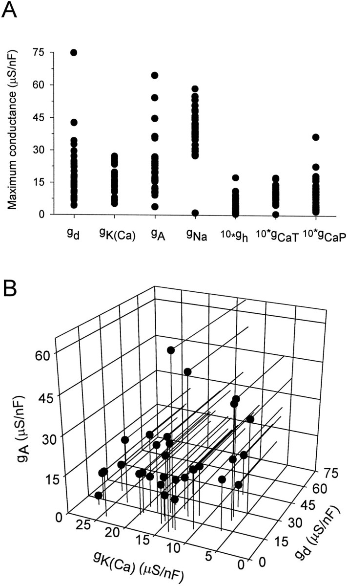
Range of equilibrium conductance values for a bursting model neuron. The model was run repeatedly starting from randomly chosen initial maximal conductance values until a steady-state pattern of bursting activity was attained. The initial maximal conductances for CaT, CaS, and_H_ were chosen uniformly in the range between 0.05 and 0.95 μS/nF, whereas the maximal conductances for the remaining active currents were chosen randomly between 2.5 and 47.5 μS/nF. The_points_ show final steady-state maximal conductances for 31 runs. A, Range of steady-state maximal conductances. Note that the maximal conductances for some of the currents have been multiplied by 10 to make them more visible. B, Maximal conductances of the three outward currents in each run plotted against each other to show that no strong correlation or pattern emerges.
The range of conductances shown in Figure 4, over which the model neuron can display bursting activity, is surprisingly large. In general, the model predicts that neurons exhibiting similar patterns of activity may, nevertheless, have significantly different maximal conductances of their membrane currents. To test this prediction we examined voltage-clamp measurements of three K+currents in the LP neuron of the crab STG (Golowasch and Marder, 1992). The LP is an identified neuron with a well defined and characteristic pattern of activity. Conductance densities of three different K+ currents, _I_Kd,_I_KCa, and_I_A, were measured in 12 neurons. Figure5A shows the values of the conductance densities measured for each of the K+currents. The variability is large. We examined the data to determine whether there are fixed ratios or other simple relationships between the conductances for the different currents. When the measured conductances are plotted against each other (Fig. 5B), no clear correlation is apparent. Interestly, no clear pattern can be seen for this set of three conductances in the model either (Fig.4B).
Fig. 5.
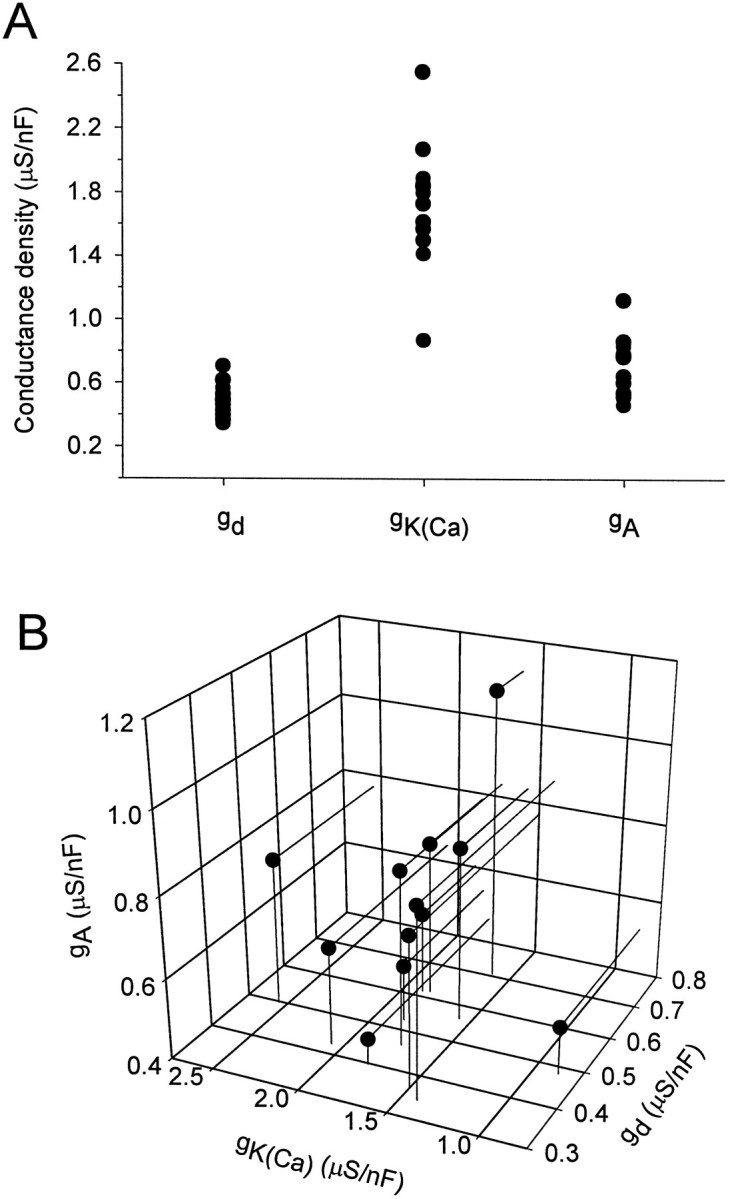
Range of conductance densities for K+ currents measured in 12 LP neurons from the crab STG. Each point represents a different neuron.A, Distribution of conductance densities measured.B, Conductance densities for the three K+ currents in individual neurons plotted against each other. As in Figure 4B, no obvious correlation or pattern can be seen.
The conductance variability seen in the LP neuron is comparable to that seen in the model. Although the relative ranges and distributions of conductance values show in Figures 4 and 5 match quite well, the magnitude of the conductances in the LP cell is significantly smaller than in the model. This is attributed, in part, to the fact that the measured values are not maximal conductances but actual conductances measured under defined conditions. Nonmaximal activation and residual inactivation in these currents under the measurement conditions may contribute to the smaller values, but the discrepancy may simply be because the model describes a different type of intrinsic activity than that exhibited by the LP neuron. The model neuron is a burster, not a model of the LP neuron that was in a tonic firing mode when the measurements were made.
Figure 6 illustrates the robustness that is the hallmark of models with activity-regulated conductances. Here a model neuron that had established a bursting pattern of activity (Fig.6A) was perturbed by changing the value of the K+ equilibrium potential,_E_K, from −80 mV to −60 mV. Such a shift could be made in a real system by changing the extracellular K+ ion concentration. This shift had, initially, a large impact on the activity of the model neuron (Fig.6B). The model sensed the resulting change in activity through the modification in the entry of Ca2+ into the cell, and it adjusted its maximal conductances until strong bursting was restored (Fig. 6C). The dominant conductance change was in _I_Na and_I_Kd, corresponding to the fact that the main effect of the perturbation was to reduce the number of action potentials being generated. Shifting _E_K back to its initial value had a similar transient effect (Fig.6D) and then resulted in a return to bursting (Fig.6E). Note, however, that the maximal conductances established at the end of this exercise are somewhat different from those initially present. In these models, the values of maximal conductances are history dependent and highly variable even though activity is robustly stable.
Fig. 6.

Response to an external perturbation.A, The model was at equilibrium producing the bursting activity shown. B, The membrane potential immediately after the reversal potential for the K+ currents was changed from −80 mV to −60 mV. C, The activity of the model after a new equilibrium configuration of maximal conductances developed in response to the perturbation. D, The membrane potential immediately after the K+ reversal potential was set back to −80 mV. E, Recovery of the model back to the initial bursting activity. The plots at the_right_ show the maximal conductances corresponding to these different cases. These are not shown for B and_D_, because they are identical, respectively, to the histograms in A and C. Note the increase in Na and K_d conductances in_C and that the conductances in A and_E_ are not identical.
We also tested the stability of the model by deleting a current after the model reached an equilibrium state. As seen in Figure7B, knocking out the membrane current _I_H greatly decreases the cycle frequency and results in weaker bursts than under steady-state conditions with_I_H present (Fig. 7A). Because of the reduction in activity seen in Figure 7B, Ca2+ entry dropped, the Ca2+sensors drifted from their equilibrium values and the maximal conductance parameters started to change. When steady-state equilibrium was restored, the model neuron had not appreciably increased its cycle frequency but had significantly increased the number and amplitude of spikes per burst. The increased spiking activity compensated for the slower cycle frequency sufficiently to allow the Ca2+ sensors to reach their equilibrium values. The bursting activity in Figure 7C is, in some sense, the best that the model can do at reproducing the activity of Figure7A when it does not have the current_I_H to work with.
Fig. 7.

Effect of removing the_I_H conductance. A, Initial activity and maximal conductances of the model at equilibrium.B, Activity of the model immediately after the_I_H conductance was set to 0. The conductance histogram at right is identical to that of_A_, except that _ḡ_H = 0.C, The new equilibrium activity and conductances established by the model.
STG neurons taken from the spiny lobster Panulirus interruptus and grown in primary cell culture exhibit a number of interesting time- and activity-dependent changes in their responses to current injection (Turrigiano et al., 1994, 1995). Initially, the cultured neurons show little active response to depolarization, but after ∼3 d in culture they typically fire action potentials in bursts arising from an oscillating underlying potential. Neurons in this condition were subjected to repeated pulses of hyperpolarizing current (Turrigiano et al., 1994). During the course of this “stimulation” the character of the bursts changed and after ∼1 hr, when the pulses were stopped, the neurons no longer displayed bursting when subjected to steady depolarizing current. Instead, they fired a steady train of action potentials. If the neurons were left unperturbed for ∼1 hr, the original pattern of bursting activity was restored.
Figure 8 shows that the model we have presented reproduces the results of these experiments. In Figure8A the model neuron is in an equilibrium bursting state that resembles the activity of the neurons studied experimentally before stimulation. Given that the membrane currents we used were based on measurements made on these neurons, this match is to be expected. Figure 8, B and C, shows what happens over time when the model is subjected to periodic hyperpolarizing current pulses. As in the experiments, the character of the bursts changes and, when the current pulses are removed, the neuron fires action potentials at a steady rate with no sign of bursting (Fig. 8D). Over time, in the absence of current injection, bursting behavior is restored (Fig. 8E) until the neuron returns to its initial equilibrium behavior (Fig. 8F). This duplication of the experimental result does not rely merely on the fact that the modeled membrane currents matched those in the real neurons. It requires the regulation process that allows activity to modify conductances to be modeled with fair accuracy as well.
Fig. 8.

Simulation of experiments done on cultured STG neurons (Turrigiano et al., 1994). A, The activity of the model neuron in its initial equilibrium configuration.B, Activity during a series of hyperpolarizing current pulses applied to the model. The injected current is plotted below the membrane potential trajectory. C, Same as_B_ but after more prolonged exposure to hyperpolarizing current pulses. D, The activity of the model immediately after the prolonged sequence of hyperpolarizing pulses was terminated.E, Activity somewhat longer after the hyperpolarizing pulses were terminated. F, Recovery of the model back to its initial state.
Because the maximal conductances in the model we have presented are dynamic variables, not fixed parameters, they cannot be adjusted by hand to coax the model into behaving in a desired manner, as is usually done in neuronal modeling. Model activity can only be controlled by adjusting the equilibrium values of the three Ca2+ sensors, F,S, and D. These represent equilibrium points for the three different signal transduction pathways, and in the model they are free parameters. The slow and fast sensor values provide the most control for changing the steady-state activity of the model. Figure 9 shows a variety of steady-state behaviors that can be achieved for different values of these parameters. The range includes tonic firing and a variety of bursting patterns.
In Figure 9, we have purposely chosen parameter values that do not cause the activity of the neuron to differ too radically from the bursting state that was considered in all the other figures. This is because the Ca2+ sensors were specifically designed to be sensitive to patterns of activity in the frequency ranges relevant for this type of bursting. If the activity of the neuron shifts to a radically different frequency range, these sensors will no longer be optimal and instability can result. Thus, shifting the activity of the neuron may require combined and concerted shifts in sensor equilibrium values and sensor dynamics. This feature may simply be a limitation of the model. Perhaps if a better or more complete set of sensors were found, they could stabilize the model for any desired pattern of activity. Alternately, neurons may develop sets of sensors that are specialized to the range of activity that they exhibit, and no “universal” set, applicable to all patterns of activity, may exist.
DISCUSSION
The standard approach to building a detailed conductance-based neuron model involves setting the maximal conductance parameters to fixed numbers that are supposed to reflect the “true” values for the neuron being modeled. A basic assumption needed to justify this procedure is that the maximal conductances of neurons are fixed quantities that have “correct” values for the model to match. The results we have presented challenge this assumption. First, the view that a given neuron has a fixed set of maximal conductances that is uniquely tied to its behavior is not supported by the model. Second, data indicate a wide range of conductance values for the identified LP neuron of the STG. Instead, we suggest that a set of biological mechanisms that control the synthesis, modulation, and degradation of membrane channels can produce the electrical characteristics required by a neuron, in a number of different ways. Therefore, an identified neuron displaying a stereotyped activity pattern, such as the LP neuron, could have significantly different sets of conductances when measured in two animals or in the same animal at two different times. Perhaps some of the variability in physiological measurements of membrane currents that has been attributed to experimental error may reflect instead an intrinsic variability inherent even in identified cell types. Rather than thinking of fixed conductances generating neuronal activity, we propose that relatively fixed average neuronal activity regulates variable conductances. Stated another way, we suggest that neurons regulate activity rather than conductances. This does not imply that there are no fixed parameters that characterize a given neuron type (our model after all has fixed parameters in it). However, the fixed parameters may not be the maximal conductances themselves, but rather parameters related to the mechanisms that control maximal conductances.
In the model presented, we have not tried to model the signal transduction pathways responsible for activity-dependent conductance regulation in any detail. Because we are predominantly interested in steady-state behavior, we could consider a linearized description around the equilibrium point of each transduction pathway. This led to the introduction of parameters describing the equilibrium points, most notable the equilibrium sensor values F,S, and D. In principle, these have a well defined meaning in terms of the biochemistry of the signal transduction pathways, but because this is unknown, they appear as free parameters in our model. We have set their values to achieve a particular type of activity. In biological neurons, these equilibrium points would be established by the basic molecular biology and biochemistry of the cell and their values would be determined as part of the process by which a neuron differentiates into a particular cell type. Specifically, these values reflect the properties of the particular Ca2+-dependent process active in each cell. Once established, fluctuations around the equilibrium points guide the construction and maintenance of membrane conductances. It is possible that modulatory processes could later change the equilibrium points leading to a fundamental change in the target pattern of activity of the neuron. Alternately, they may be fixed for the life of the cell once it differentiates.
We used three different Ca2+ sensors as the feedback elements in the model, but the fact that we still did not obtain complete stability suggests that more than three elements may be required. Given the complexities of cellular signal transduction, we would expect a significant number of different pathways, certainly more than the three we have modeled (Bitu et al., 1997). Some pathways may integrate Ca2+ and other second messenger signals slowly to regulate gene expression and channel synthesis (Fields et al., 1997). Others may act over a more rapid time scale controlling, for example, insertion of channels into the cell membrane and channel cross-linking to the cytoskeleton. Finally, other pathways could control levels of channel phosphorylation (Levitan, 1994). It is not essential that all, or indeed any, of the pathways involve intracellular Ca2+. Any other second messenger that links the molecular biology inside the neuron to the behavior of the membrane potential will suffice. However, considering the widespread role of Ca2+ as a second messenger, it seems likely that Ca2+ plays at least some role in the processes we are modeling.
The modification of intrinsic membrane conductances by activity adds a new element to the type of plasticity normally considered in neuronal circuit models. Activity is known to mediate many processes, including changes in synaptic efficacy (Artola and Singer, 1993; Bliss and Collingridge, 1993; Malenka and Nicoll, 1993) (Turrigiano et al., 1998) and neurite outgrowth (Fields et al., 1990; Kater and Mills, 1991; van Ooyen and van Pelt, 1994) in addition to modifying ionic currents. This raises interesting possibilities for modeling the growth and development of neural circuits (Casey et al., 1997; Jensen and Abbott, 1997) including the effects of activity on intrinsic neuronal properties, axonal and dendritic growth, synaptogenesis, and synaptic strength.
The membrane potential V of the model neuron is computed by numerically integrating the equation:
in which the currents _I_i are given by Equation 1 and the sum over i refers to the eight currents of the model (seven voltage-dependent and one leak). The values of the parameters p and E for the different currents are given in Figure 10. In all cases, the value of q was either 0 or 1. Cases with q = 0 can be identified from Figure 10, because no_h_∞ or τh functions are listed for them. In addition to the currents listed in Figure 10, there is a leakage conductance with p = q = 0, _ḡ_leak = 0.01 μS/nF, and_E_leak = −50 mV. All maximal conductances are normalized to the surface area of the neuron by dividing the total conductance by the capacitance of the neuron, so their units are μS/nF. No values for the maximal conductances of other currents are given because these are dynamical variables, not model parameters. The value for the reversal potential for Ca2+ currents is not given in Figure 10, because it was computed from the intracellular Ca2+ concentration using the Nernst equation with an external Ca2+ concentration of 3 mm.
Fig. 10.

Parameters and functions used to describe the membrane currents of the model. Notation is explained in the text. All membrane potentials are in millivolts, time constants are in milliseconds, and [Ca] refers to the micromolar intracellular Ca2+ concentration.
The activation and inactivation variables _m_i and_h_i are computed by numerically integrating equations of the form: Eq. pg 33 bottom
The functions _m_∞, τm, _h_∞, and τh are given in Figure 10. Note that_m_∞ for the current _I_KCadepends on the Ca2+ concentration as well as on the voltage. The calcium concentration, used to control_I_KCa, is determined by integrating the equation
=−(0.94 μM·nF/nA)ICa−[Ca2+]+0.05 μM
reflecting the fact that the total Ca2+ current determines how much Ca2+ enters the cell and assuming that Ca2+ is removed, sequestered, and buffered at a rate that depends linearly on the Ca2+concentration. We set the time constant for Ca2+removal to be 20 msec. The factor that multiplies_I_Ca depends on the ratio of the surface area of the cell to the volume in which the Ca2+concentration is measured. We have taken this volume to be a narrow shell just inside the membrane and approximated the neuron by a cylinder 50 μm in diameter and 400 μm long. This gives a capacitance of 0.628 nF. The last term on the right side of this equation sets the value of the resting Ca2+concentration.
Footnotes
This work was supported by the Sloan Center for Theoretical Neurobiology at Brandeis University, National Institute of Mental Health Grant MH46742, the McKnight Foundation, and the W. M. Keck Foundation. We thank Mark Goldman for helpful consultation.
Correspondence should be addressed to Larry Abbott, Volen Center, MS 013, Brandeis University, 415 South Street, Waltham, MA 02254.
REFERENCES
- 1.Abbott LF, LeMasson G. Analysis of neuron models with dynamically regulated conductances. Neural Comp. 1993;5:823–842. [Google Scholar]
- 2.Alkon DL. Calcium-mediated reduction of ionic currents: a biophysical memory trace. Science. 1984;226:1037–1045. doi: 10.1126/science.6093258. [DOI] [PubMed] [Google Scholar]
- 3.Artola A, Singer W. Long-term depression of excitatory synaptic transmission and its relationship to long-term potentiation. Trends Neurosci. 1993;16:480–487. doi: 10.1016/0166-2236(93)90081-v. [DOI] [PubMed] [Google Scholar]
- 4.Bito H, Deisseroth K, Tsien RW. Ca2+-dependent regulation in neuronal gene expression. Curr Opin Neurobiol. 1997;7:419–429. doi: 10.1016/s0959-4388(97)80072-4. [DOI] [PubMed] [Google Scholar]
- 5.Bliss TVP, Collingridge GL. A synaptic model of memory: long-term potentiation in the hippocampus. Nature. 1993;361:31–39. doi: 10.1038/361031a0. [DOI] [PubMed] [Google Scholar]
- 6.Casey M, Golowasch J, Abbott LF, Marder E. Activity-dependent regulation of network activity: theoretical and experimental approach. Soc Neurosci Abstr. 1997;23:476. [Google Scholar]
- 7.Fields RD, Neale EA, Nelson PG. Effects of patterned electrical activity on neurite outgrowth from mouse neurons. J Neurosci. 1990;10:2950–2964. doi: 10.1523/JNEUROSCI.10-09-02950.1990. [DOI] [PMC free article] [PubMed] [Google Scholar]
- 8.Fields RD, Eshete F, Stevens B, Itoh K. Action potential dependent regulation of gene expression: temporal specificity in Ca2+ cAMP-responsive element binding proteins, and mitogen-activated protein kinase signaling. J Neurosci. 1997;17:7252–7266. doi: 10.1523/JNEUROSCI.17-19-07252.1997. [DOI] [PMC free article] [PubMed] [Google Scholar]
- 9.Franklin JL, Fickbohm DJ, Willard AL. Long-term regulation of neuronal calcium currents by prolonged changes of membrane potential. J Neurosci. 1992;12:1726–1735. doi: 10.1523/JNEUROSCI.12-05-01726.1992. [DOI] [PMC free article] [PubMed] [Google Scholar]
- 10.Gallin WJ, Greenberg ME. Calcium regulation of gene expression in neurons: the mode of entry matters. Curr Opin Neurobiol. 1995;3:367–374. doi: 10.1016/0959-4388(95)80050-6. [DOI] [PubMed] [Google Scholar]
- 11.Golowasch J, Marder E. Ionic currents of the lateral pyloric neuron of the stomatogastric ganglion of the crab. J Neurophysiol. 1992;67:318–331. doi: 10.1152/jn.1992.67.2.318. [DOI] [PubMed] [Google Scholar]
- 12.Gu X, Spitzer N. Distinct aspects of neuronal differentiation encoded by frequency of spontaneous Ca2+ transients. Nature. 1995;375:784–787. doi: 10.1038/375784a0. [DOI] [PubMed] [Google Scholar]
- 13.Hodgkin AL, Huxley AF. A quantitative description of membrane current and its application to conduction and excitation in nerve. J Physiol (Lond) 1952;117:500–544. doi: 10.1113/jphysiol.1952.sp004764. [DOI] [PMC free article] [PubMed] [Google Scholar]
- 14.Hong SJ, Lnenicka GA. Activity-dependent reduction in voltage-dependent calcium current in a crayfish motoneuron. J Neurosci. 1995;15:3539–3547. doi: 10.1523/JNEUROSCI.15-05-03539.1995. [DOI] [PMC free article] [PubMed] [Google Scholar]
- 15.Hong SJ, Lnenicka GA. Characterization of a P-type calcium current in a crayfish motoneuron and its selective modulation by impulse activity. J Neurophysiol. 1997;77:76–85. doi: 10.1152/jn.1997.77.1.76. [DOI] [PubMed] [Google Scholar]
- 16.Hooper SL, O’Neil M, Wagner R, Ewer J, Golowasch J, Marder E. The innervation of the pyloric region of the crab, Cancer borealis: homologous muscles in decapod species are differently innervated. J Comp Physiol [A] 1986;159:227–240. doi: 10.1007/BF00612305. [DOI] [PubMed] [Google Scholar]
- 17.Jensen O, Abbott LF. Self-organizing circuits of model neurons. In: Bower J, editor. Computational Neuroscience, Trends in Research. Plenum; New York: 1997. pp. 227–230. [Google Scholar]
- 18.Kater SB, Mills LR. Regulation of growth cone behavior by calcium. J Neurosci. 1991;11:891–899. doi: 10.1523/JNEUROSCI.11-04-00891.1991. [DOI] [PMC free article] [PubMed] [Google Scholar]
- 19.LeMasson G, Marder E, Abbott LF. Activity-dependent regulation of conductances in model neurons. Science. 1993;259:1915–1917. doi: 10.1126/science.8456317. [DOI] [PubMed] [Google Scholar]
- 20.Levitan I. Modulation of ion channels by protein phosphorylation. Annu Rev Physiol. 1994;56:193–212. doi: 10.1146/annurev.ph.56.030194.001205. [DOI] [PubMed] [Google Scholar]
- 21.Li M, Jia M, Fields RD, Nelson PG. Modulation of calcium currents by electrical activity. J Neurophysiol. 1996;76:2595–2607. doi: 10.1152/jn.1996.76.4.2595. [DOI] [PubMed] [Google Scholar]
- 22.Linsdell P, Moody WJ. Electrical activity and calcium influx regulate ion channel development in embryonic Xenopus skeletal muscle. J Neurosci. 1995;15:4507–4514. doi: 10.1523/JNEUROSCI.15-06-04507.1995. [DOI] [PMC free article] [PubMed] [Google Scholar]
- 23.Malenka RC, Nicoll RA. NMDA-receptor-dependent synaptic plasticity: multiple forms and mechanisms. Trends Neurosci. 1993;16:521–527. doi: 10.1016/0166-2236(93)90197-t. [DOI] [PubMed] [Google Scholar]
- 24.Marder E, Eisen JS. Transmitter identification of pyloric neurons: electrically coupled neurons use different neurotransmitters. J Neurophysiol. 1984;51:1345–1361. doi: 10.1152/jn.1984.51.6.1345. [DOI] [PubMed] [Google Scholar]
- 25.Marder E, Abbott LF. Theory in motion. Curr Opin Neurobiol. 1995;5:832–840. doi: 10.1016/0959-4388(95)80113-8. [DOI] [PubMed] [Google Scholar]
- 26.Murphy TH, Worley PF, Baraban JM. L-type voltage-sensitive calcium channels mediate synaptic activation of immediate early genes. Neuron. 1991;7:625–635. doi: 10.1016/0896-6273(91)90375-a. [DOI] [PubMed] [Google Scholar]
- 27.Ross WM. Changes in intracellular calcium during neuron activity. Annu Rev Physiol. 1989;51:491–506. doi: 10.1146/annurev.ph.51.030189.002423. [DOI] [PubMed] [Google Scholar]
- 28.Siegel M, Marder E, Abbott LF. Activity-dependent current distributions in model neurons. Proc Natl Acad Sci USA. 1994;91:11308–11312. doi: 10.1073/pnas.91.24.11308. [DOI] [PMC free article] [PubMed] [Google Scholar]
- 29.Turrigiano G, Abbott LF, Marder E. Activity-dependent changes in the intrinsic electrical properties of cultured neurons. Science. 1994;264:974–977. doi: 10.1126/science.8178157. [DOI] [PubMed] [Google Scholar]
- 30.Turrigiano G, LeMasson G, Marder E. Selective regulation of current densities underlies spontaneous changes in the activity of cultured neurons. J Neurosci. 1995;15:3640–3652. doi: 10.1523/JNEUROSCI.15-05-03640.1995. [DOI] [PMC free article] [PubMed] [Google Scholar]
- 31.Turrigiano G, Leslie K, Desci N, Rutherford L, Nelson SB (1998) Activity-dependent scaling of quantal amplitude in neocortical neurons. Nature, in press. [DOI] [PubMed]
- 32.van Ooyen A, van Pelt J. Activity-dependent outgrowth of neurons and overshoot phenomena in developing neural networks. J Theor Biol. 1994;167:27–44. [Google Scholar]