Orientation Selectivity and the Arrangement of Horizontal Connections in Tree Shrew Striate Cortex (original) (raw)
Abstract
Horizontal connections, formed primarily by the axon collaterals of pyramidal neurons in layer 2/3 of visual cortex, extend for millimeters parallel to the cortical surface and form patchy terminations. Previous studies have provided evidence that the patches formed by horizontal connections exhibit modular specificity, preferentially linking columns of neurons with similar response characteristics, such as preferred orientation. The issue of how these connections are distributed with respect to the topographic map of visual space, however, has not been resolved. Here we combine optical imaging of intrinsic signals with small extracellular injections of biocytin to assess quantitatively the specificity of horizontal connections with respect to both the map of orientation preference and the map of visual space in tree shrew V1. Our results indicate that horizontal connections outside a radius of 500 μm from the injection site exhibit not only modular specificity, but also specificity for axis of projection. Labeled axons extend for longer distances, and give off more terminal boutons, along an axis in the map of visual space that corresponds to the preferred orientation of the injection site. Inside of 500 μm, the pattern of connections is much less specific, with boutons found along every axis, contacting sites with a wide range of preferred orientations. The system of long-range horizontal connections can be summarized as preferentially linking neurons with co-oriented, co-axially aligned receptive fields. These observations suggest specific ways that horizontal circuits contribute to the response properties of layer 2/3 neurons and to mechanisms of visual perception.
Keywords: orientation selectivity, topography, optical imaging, visual cortex, surround effects, tree shrew, biocytin, horizontal connections
Horizontal connections are a prominent feature of the intrinsic circuitry of the visual cortex. These connections originate primarily from pyramidal cells, extend for 2–5 mm parallel to the cortical surface, and terminate in a highly selective and patchy manner (Gilbert and Wiesel, 1979, 1983; Rockland and Lund, 1982). A number of experiments have focused on the relationship between the patches formed by horizontal connections and well known modular features of cortical organization such as orientation columns, ocular dominance columns and cytochrome oxidase-rich blobs (Livingstone and Hubel, 1984; T’so et al., 1986; Gilbert and Wiesel, 1989; Malach et al., 1993). The results from these experiments suggest that the patchy nature of horizontal connections can be explained by a simple rule: horizontal connections link together select subsets of neurons that share similar receptive field properties. Studies in both cat and monkey visual cortex, for example, have shown that horizontal connections selectively link patches of neurons that have similar orientation preferences (Gilbert and Wiesel, 1989; Malach et al., 1993).
The relationship of horizontal connections to another fundamental aspect of cortical organization—the orderly map of visual space—is less clear. This issue is of interest because the axon arbors of individual neurons are often elongated across the cortical surface, extending further and giving rise to more terminals along one axis of the map than others (Gilbert and Wiesel, 1983, 1989; Matsubara et al., 1985, 1987; McGuire et al., 1991; Kisvarday and Eysel, 1992;Amir et al., 1993, Malach et al., 1993). Furthermore, the results of several physiological and perceptual studies have led to the suggestion that the effects mediated by horizontal connections are not distributed randomly about a point in visual space, but are aligned along an axis that corresponds to a neuron’s preferred orientation. For example, a collinear arrangement of horizontal connections has been implicated in the construction of the elongated receptive fields of layer 6 neurons in cat striate cortex (Bolz and Gilbert, 1989). Likewise, perceptual studies of contour integration and physiological studies of receptive field surround effects in layer 2/3 neurons have provided evidence for facilitatory effects that are much stronger in regions of visual space that lie along the axis of preferred orientation than in regions that lie off this axis (Nelson and Frost, 1985; Fiorani et al., 1992; Field et al., 1993; Polat and Sagi, 1993; Kapadia et al., 1995). Despite the evidence for anisotropic physiological and psychophysical effects, the relationship between the axis of elongation of horizontal connections and the orientation preference of the neurons they interconnect has never been systematically examined.
In the experiments described here, we have combined optical imaging of intrinsic signals with small extracellular injections of biocytin to quantitatively assess both the modular and axial arrangement of horizontal connections established by neurons of known orientation preference in layer 2/3 of tree shrew striate cortex. Our results demonstrate a remarkable degree of specificity for both features of horizontal connectivity, and suggest several ways that horizontal connections could contribute to the response properties of layer 2/3 neurons.
MATERIALS AND METHODS
Experimental design. Small extracellular injections of biocytin were made in 13 animals. Distributions of labeled boutons resulting from the injections were plotted and analyzed manually (3 cases) or with the assistance of a computer reconstruction system and software routines written in our lab (10 cases, see below for details). Analysis of modular specificity of the bouton distributions was accomplished in 7 of these 10 cases by using optical imaging of intrinsic signals to determine the map of orientation preference in V1 before injection of the biocytin. Analysis of the bouton distributions with respect to the map of visual space was accomplished in all 13 of the cases. Optical imaging was also used to investigate the geometry of the map of visual space in three animals that were not used for analysis of specificity of connections.
Animal surgery. Tree shrews were initially anesthetized with a mixture of ketamine hydrochloride (200 mg/kg) and xylazine (4.7 mg/kg) given by intramuscular injection. Atropine sulfate (0.08 mg) was given sub-cutaneously to reduce secretions. An intraperitoneal cannula was inserted, the trachea intubated, and the animal was placed in a modified stereotaxic frame allowing unobstructed viewing of the stimulus monitor. During surgery, anesthesia was maintained with a 2:1 mixture of N2O/O2 supplemented with 2% halothane. Body temperature was maintained with a thermostatically controlled heating blanket. The eyes were kept moist by using planar contact lenses. An incision was made in the scalp, muscle and fascia reflected, and the bone overlying visual cortex was thinned by scraping with a fine scalpel. Wound margins and incisions were treated with a long-acting local anesthetic (bupivacaine) and pressure points were treated with a lidocaine ointment. The animal was paralyzed using pancuronium bromide (0.8 mg initial dose for first 1.5 hr, then 0.2 mg/hr) administered through the intraperitoneal cannula to prevent eye movements, and artificially respired at a rate and volume sufficient to maintain expired CO2 at 3–4%. During optical imaging, halothane levels were reduced to 1%, and the N2O/O2 mixture to 1:1. Any signs of distress evident in the electrocardiogram or expired CO2 were treated by immediately increasing the level of halothane.
Optical imaging. Optical imaging of intrinsic signals was accomplished using an enhanced video acquisition system (Optical Imaging Inc.) applying techniques similar to those of Grinvald and colleagues (Grinvald et al., 1986; Bonhoeffer and Grinvald, 1991,1993). Images were obtained directly through the thinned bone overlying the V1 area. The cortex was illuminated with orange light (605 nm) and visualized with a tandem lens macroscope attached to a low noise video camera. Visual stimulation for optical imaging was provided by a separate stimulus computer (386 PC with SGT+ graphics board and STIM software provided by Kaare Christian). The stimuli used consisted of high-contrast square wave gratings (6.25° dark phase, 1.25° light phase, drifted at 22.5°/sec). Four gratings of orientation 0°, 45°, 90°, and 135° with respect to horizontal were used. Each grating was moved back and forth along an axis that was orthogonal to the orientation of the grating. Data were acquired during between 20 and 80 presentations of each stimulus. The summed images acquired during the presentation of one grating were subtracted from the summed images acquired during presentation of the orthogonal grating to create differential maps of orientation preference (difference images), (Blasdel, 1992). Difference images were 655 × 480 pixels in resolution, with either 62 or 75 pixels per millimeter depending on the lens combination used. Resulting difference images were smoothed using a 7 × 7 pixel mean filter kernel. Low frequency noise was reduced by convolving the image with a 40 × 40 pixel mean filter kernel and subtracting the result from the original image. Difference images were normalized by dividing the deviation from the mean at each pixel by the average absolute deviation across the entire image (Weliky et al., 1995). Finally, vector summation of the difference images was done on a pixel by pixel basis to create a color coded orientation preference map(Bonhoeffer and Grinvald, 1991,1993; Blasdel, 1992).
Optical imaging of the geometry of the map of visual space in V1 was accomplished using procedures similar to those developed by Campbell and Blasdel (1995). The technique uses difference imaging for spatial location to identify areas of cortex that respond preferentially to stimulation of a particular line in visual space. The stimuli used consisted of two gratings of the same orientation, each with a period of 10° but differing in the width and spatial location of the light phase of the grating (grating 1 = 1° light phase, 9° dark phase; grating 2 = 3° light phase, 7° dark phase). The two gratings were placed and moved in such a way that the light phases of the gratings covered non-overlapping regions of the stimulus monitor (grating 1 moved ±1° from original position, grating 2 moved ±2° from original position). Images acquired during presentation of grating 2 were subtracted from images acquired during presentation of grating 1 for each orientation to create topographic difference images. Topographic difference images were smoothed with a 7 × 7 pixel mean filter kernel for presentation.
At the conclusion of the optical imaging phase of the experiment, a_reference image_ of the surface blood vessels was acquired, while the cortex was illuminated with green (540 nm) light.
Biocytin injections. Injection sites were selected by examining the difference images and orientation preference maps to find an area of relatively constant orientation preference. Selected sites were located using blood vessels visible in the reference image and on the cortical surface as seen under a surgical microscope. The orientation tuning of the injection site was confirmed by recording multi-unit activity through the injection micropipette. Tuning curves were obtained by averaging responses from 5–8 trials of 9 oriented stimuli. Iontophoretic injections were made with glass micro pipettes with a tip diameter of ∼10 μm containing 5% biocytin (Sigma, St. Louis, MO) in saline using pulsed current (7 sec on, 7 sec off) of 2.5 μamps for 10–15 min. After the injection the animal was sutured, recovered from paralytic and anesthesia, and returned to its cage.
Tissue processing. After a 16 hr recovery period, the animal was deeply anesthetized with Nembutal (25 mg, i.p.) and transcardially perfused with 0.9% saline, followed by 10% formalin in 0.1m sodium phosphate buffer. The brain was removed and a block of cortex containing V1 was flattened while immersed in 20% sucrose in 0.1 m sodium phosphate buffer and maintained at 4°C overnight. The following day 40 μm tangential sections were cut from the block on a freezing microtome. Care was taken to collect a first section that contained outlines of the surface vasculature, so that the tissue sections could later be aligned with the reference image. Our procedures for visualization of the biocytin label have been published (Usrey and Fitzpatrick, 1996). Briefly, goat anti-biotin and biotinylated rabbit anti-goat antibodies (Vector Laboratories, Burlingame, CA) were used to amplify the signal before processing with the standard avidin–biotin complex (Vectastain Kit PK-4000, Vector, Burlingame, CA) reaction, and diaminobenzidine with nickel and cobalt intensification. Visualization of the V1/V2 border was accomplished by using a Nissl counterstain. Some sections were counterstained before they were coverslipped, and some sections were counterstained after bouton distributions were plotted.
Bouton plotting, alignment, and analysis. Blood vessel outlines in the first tissue section, radial vessel profiles, and labeled boutons from 2–6 sections were plotted using Neurolucida software (Microbrightfield, Colchester, VT). In each case, enough sections were plotted to assess the bouton distribution in the superficial layers throughout the dorsal region of V1. The data were stored as a series of x,y coordinates for each bouton or each blood vessel reference point in the slice. These data were aligned with the optical imaging data using software routines written as an extension to the public domain National Institutes of Health Image program [original version written by Wayne Rasband at National Institutes of Health and available from Internet by anonymous ftp from zippy.nimh.nih.gov or on floppy disk from NTIS (5285 Port Royal Rd., Springfield, VA 22161, part number PB93–504868)]. The first stage of the alignment was to align the computer drawing of the first tissue section to the reference image acquired during optical imaging. Global scaling, rotation, and x,_y_translations were applied to the stored coordinates to achieve the best overall alignment possible, with emphasis placed on the area of the slice containing the injection and bouton data. The second stage of the alignment was to align deeper tissue sections, containing labeled boutons, to an overlay of the first section drawing and reference image by using the profiles of blood vessels that course radially through V1. As in the first stage, only global scaling, rotation, and translations were used to align the section. At the end of this procedure, the same transformations used to align the blood vessel reference points in deep sections were then applied to the bouton data (coordinates). This allowed direct comparison of the bouton distributions with the map of orientation preference, which was in the exact same field of view as the reference image. Bouton distributions were not compared with the map of orientation preference until the completion of the alignment process.
Bouton tuning curves were obtained by counting the number of boutons that contacted sites with various orientation preferences using 10° bins of orientation preference. Bouton tuning curves were computed separately for boutons that were greater or less than 500 μm from the injection site. Axial specificity was assessed by counting the number of boutons within each 10° sector around the injection site, excluding the boutons that were within 500 μm of the injection site. Profiles showing the number of boutons versus distance were obtained for both preferred and orthogonal axes (±30°). Maximum distance of projection along the preferred and orthogonal axes were determined by calculating the maximum distance that a minimum density of 40 boutons/0.01 mm2 could be found.
Three of the cases used for determination of axial specificity were plotted using an alternative system that did not allow the use of the extended National Institutes of Health Image routines for alignment and analysis. For these cases, the bouton distribution was plotted from superficial sections containing layer 2/3, and the V1/V2 border was plotted in thionin stained sections from layer 4. The border was then transferred to the layer 2/3 plots by using the position of radial blood vessel profiles. The number of boutons within 10° sectors around the injection site was then counted manually. Similar results were obtained by both methods, but density, distance profiles, and maximum distance calculations were not attempted using the manual counting method.
RESULTS
In the next sections, we describe the results from experiments designed to examine the distribution of biocytin-labeled terminals with respect to the map of orientation preference and the map of visual space in striate cortex (V1) of the tree shrew. In the first section we begin by considering the basic features of the orientation preference map that are relevant for understanding the quantitative assessment of modular specificity.
Maps of orientation preference in tree shrew striate cortex
Previous studies demonstrated that neurons in the superficial layers of tree shrew striate cortex are sharply tuned to the orientation of edges (Humphrey et al., 1980a); moreover, on the basis of 2-deoxyglucose (2-DG) labeling, it was suggested that neurons with similar orientation preferences were arranged in a series of parallel bands or stripes that intersected the V1/V2 border at right angles (Humphrey et al., 1980b). If the 2-DG experiments have provided an accurate picture of the layout of iso-orientation domains, then the map of orientation preference in the tree shrew would be considerably different from what has been described in monkeys and cats (Bonhoeffer and Grinvald, 1991, 1993; Blasdel, 1992). However, the difference could also be attributed to the fact that the results in these other species are based on more recently developed optical imaging techniques. These techniques provide a more detailed assessment of the map because they permit the comparison of the patterns of activity evoked by multiple stimulus orientations in the same region of cortex. A complete analysis of the map of orientation preference in the tree shrew striate cortex based on optical imaging techniques will be presented elsewhere; here we simply describe the basic features of the map and emphasize that the arrangement of orientation preference maps in the striate cortex of the tree shrew, monkey, and cat are fundamentally similar. Orientation selectivity was also observed in V2 of some animals, although the signal strength in V2 was much weaker for reasons that remain unknown. The functional organization of orientation selectivity and connections in V2 are not explored in this paper.
Our optical imaging experiments confirm some of the features described in the 2-DG experiments. For example, in almost all of the orientation difference images, we found regions of the cortex that had the appearance of parallel alternating dark and light stripes (Fig.1A). These stripes were common in the most caudal part of the exposed surface and along the V1/V2 border where they intersected the border at right angles. However, other parts of the map were decidedly less stripe-like in appearance; in the center of the exposed surface, for example, the stripes were often replaced by a less regular and more punctate set of domains. Furthermore, a comparison of the patterns of activity evoked by different stimulus orientations revealed that even those regions of the map that had a stripe-like appearance in images generated for one stimulus orientation would often appear to break up into discontinuous patches in images generated for other stimulus orientations. Taken together, these observations suggested that the map of orientation preference in the tree shrew is far more complex than was indicated by the earlier 2-DG experiments.
Fig. 1.
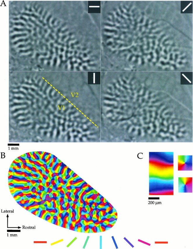
Optical imaging of intrinsic signals in tree shrew visual cortex. A, Difference images obtained for four stimulus angles (0°, 45°, 90°, 135°, shown in_inset_ of each panel) from one animal. _Black areas_of each panel indicate areas of cortex that were preferentially activated by a given stimulus, and _light gray areas_indicate areas that were active during presentation of the orthogonal angle. The dashed line in the 90° panel indicates the approximate location of the V1/V2 border. B, Orientation preference map obtained by vector summation of data obtained for each angle. Orientation preference of each location is color-coded according to the key shown below. C, Common features of the orientation preference maps. Portions of the orientation preference map shown in B have been enlarged to demonstrate that the orientation preference maps contained both linear zones (left) and pinwheel arrangements (right).
The fine-scale mapping of orientation preference is best appreciated by combining the individual difference images using vector summation to create an orientation preference map where colors are used to represent the preferred orientation at each site (Fig. 1B). This analysis confirms that the map of orientation preference in the tree shrew has the same basic organizational features that have been described previously in monkey and cat striate cortex (Bonhoeffer and Grinvald, 1991, 1993; Blasdel, 1992). In many regions of the map, commonly referred to as pinwheels, a continuous shift in orientation preference is obtained by sampling around a point, or singularity. Examples of two pinwheels from the orientation preference map shown in Figure 1B are shown at higher magnification in Figure1C. Linear zones, regions of the map in which a progressive change in orientation preference is obtained by sampling along a straight line (Blasdel, 1992; Obermayer and Blasdel, 1993), are also a prominent feature of orientation preference maps in the tree shrew. As predicted from the difference images, linear zones are common along the V1/V2 border and along the caudal edge of the dorsal portion of V1. They can extend for 2–3 mm, a distance that covers several full repeats of the orientation cycle. In Figure 1, A and_B_, an especially large linear zone is visible in the caudal portion of the map, and this same linear zone has been enlarged in the left hand side of Figure 1C.
Modular specificity of horizontal connections
To assess the modular specificity of horizontal connections, combined optical imaging and biocytin injection experiments were accomplished in seven animals. After the optical imaging phase of the experiment, an injection site was selected and the orientation tuning of the injection site was confirmed by recording multi-unit activity through the injection pipette. Our biocytin injections resulted in the labeling of a small number of cell bodies (12–65) that were confined to sites that were typically less than 200 μm in diameter (average diameter 176 μm, largest diameter 320 μm; see Fig.2A,B). In two of our cases, one or two retrogradely labeled cells could be found at some distance from the injection site, but this did not hamper our ability to detect the underlying specificity of the connections. The axonal processes of the labeled neurons were well labeled (Fig. 2C) and exhibited the characteristic bouton terminal swellings that have been described in other species (Gilbert and Wiesel, 1983; Amir et al., 1993; Kisvarday and Eysel, 1992). As seen in Figure2A, labeled axons extended away from the injection site for several millimeters and gave rise to prominent patches. Borders of bouton patches were determined subjectively and by thresholding a density plot of the bouton distributions. The two methods were in good agreement and the average size of bouton patches was determined to be ∼400 μm × 250 μm. This information is provided for comparison with other reports only; the borders of bouton patches were not used in the analysis of modular or axial specificity. The distribution of labeled boutons was plotted from between two and six sections for each case.
Fig. 2.

Biocytin injections made into superficial layers of V1. A, Low-power image showing an injection site, labeled axons leaving the site, and several patches formed by axon arbors. Radial vessel profiles used in aligning tissue sections are also visible. Scale bar, 100 μm. B, The same injection site seen in A shown at higher power. Individual cells that have taken up the biocytin can be identified. Scale bar, 25 μm.C, A patch of biocytin label shown at higher magnification. Labeled boutons are visible on the axons. Scale bar, 25 μm.
The interpretation of our findings rests on the accuracy with which we are able to align plots of labeled boutons from the anatomical sections with optical maps of orientation preference. For this reason, the steps in the alignment process are illustrated in Figure 3. This first stage of the alignment process was to align a drawing of the blood vessels found in the first section (shown in yellow in Fig. 3A) to the reference image taken during the optical imaging session (grayscale image in the_background_ of Fig. 3A). The second stage consisted of aligning deeper sections (shown in blue in Fig.3A), that contained labeled boutons, to the first section using profiles of blood vessels that course radially through the depth of the cortex. Only global scaling, translation and rotation operations were used during both stages of the alignment (no regional alignments were made and no morphing of the data were used). Emphasis was placed on getting the best alignment for the area of the sections that contained the injection site and labeled boutons. The inset of Figure3A demonstrates the degree of accuracy we were able to achieve in this process. Based on overlays such as those in Figure 3 we estimate errors in alignment of up to 50–100 μm at specific locations far removed from the injection sites, but no systematic errors throughout the section. After the alignment procedure, difference images or orientation preference maps were substituted for the reference image, and the actual bouton distribution was substituted for the blood vessel pattern.
Fig. 3.
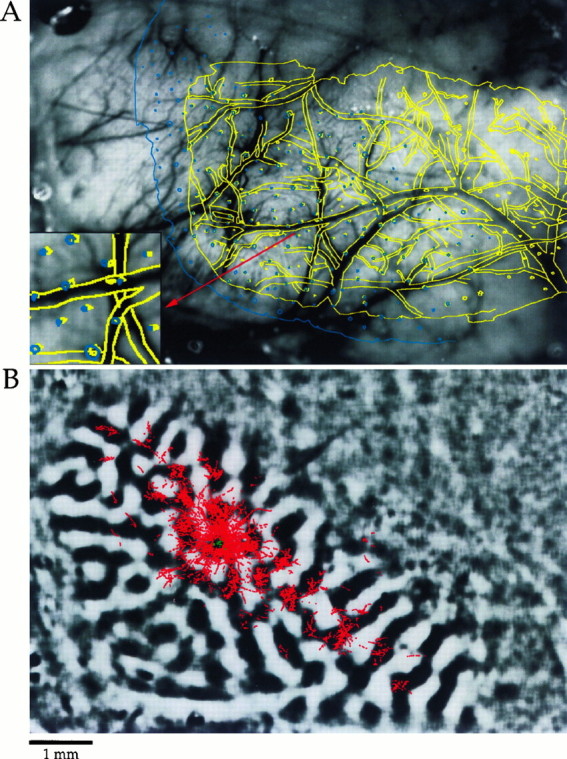
Alignment of bouton distributions to optical imaging data (case 9509). A, The image in the_background_ is a reference image taken during the optical imaging phase of the experiment. The yellow overlay is a computer-assisted drawing of blood vessel outlines and radial vessel profiles seen in the first tissue section. The drawing has been scaled, rotated, and translated to align with the reference image. The_blue overlay_ is a computer-assisted drawing of radial vessel profiles and the section outline from a deeper section that contained labeled boutons. This section has been independently scaled, rotated, and translated to align with the reference image and the first tissue section. The precision of both stages of the alignment can be seen in the inset. B, Same animal and field of view as seen in A. The reference image has been replaced with a difference image showing areas active for a 90° stimulus in black. Bouton distribution information has been added using the same transforms used to align the blue section in A. The green symbols indicate cells that took up and transported the biocytin. Red symbols_indicate locations of labeled boutons. Scale bar, 400 μm for_inset in A.
Figure 3B shows the results of the alignment process presented in Figure 3A. The injection in this case was made into a site that responded preferentially to edges with an orientation near vertical. The tuning curve based on multi-unit activity showed a peak at 80° and a half width at half height of 19°. The distribution of labeled boutons that resulted from the injection is shown superimposed on a difference image in which black regions represent areas that were strongly activated by a vertical stimulus (90°) and white regions represent areas that were strongly activated by a horizontal stimulus (0°). Except for the region immediately adjacent to the injection site, there is a striking correspondence between the distribution of labeled terminals and the regions of the orientation map that respond strongly to vertical edges.
A better appreciation of the range of orientation preferences of the sites contacted by a given set of horizontal connections can be gained by examining the bouton distributions displayed over a color-coded orientation preference map. Figure 4_A_illustrates this comparison for the same case that is depicted in Figure 3 (preferred orientation of the injection site = 80°); Figure 4B illustrates a case in which an injection was made into a site with a preferred orientation near horizontal (peak of tuning curve 160°, half-width at half-height 28.5°). In each case, beyond the area immediately adjacent to the injection site, the labeled boutons are clustered in regions that have orientation preferences similar to that of the injection site.
Fig. 4.
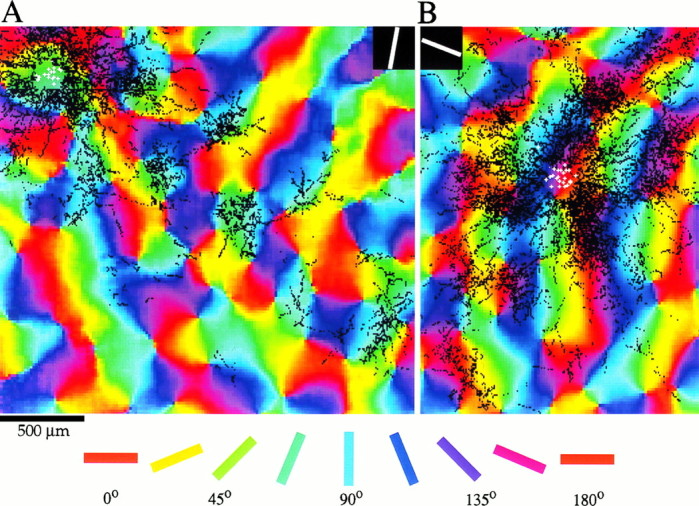
Bouton distributions shown over orientation preference maps for two cases. A, Bouton distribution after an injection into a site with a preferred orientation of 80°, determined by recording through the same tip used to make the injection (same case as in Fig. 3). The white symbols indicate the location of cells that took up the biocytin. Labeled boutons (black symbols) are found at sites with all orientation preferences near the injection site, but preferentially at sites with the same orientation preference as the injection site at longer distances. B, Results from an experiment in which an injection was made into a site with an orientation preference of 160° (case 9517). Color key and scale bar apply to both figures.
To quantify the relationship between the bouton distributions and the orientation preference maps, we generated “bouton tuning curves” that show the number of labeled boutons that overlie a particular range of orientation values in the orientation preference map. In each case examined, the bouton tuning curves for boutons found at distances greater than 500 μm from the injection site showed a clear peak at or near the preferred orientation of the injection site (Fig.5). In general, the tuning curves for boutons found at distances less than 500 μm from the injection site were considerably broader (Fig. 5A,B) but, in some cases, specificity for sites that were at or near the preferred orientation was still present (Fig. 5C).
Fig. 5.
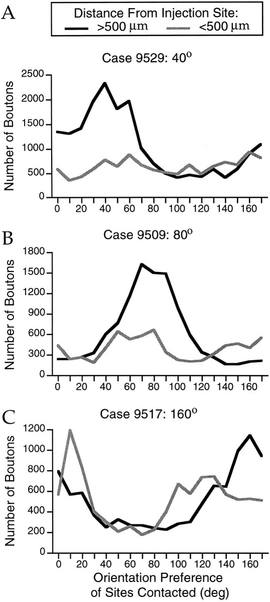
Quantitative analysis of modular specificity of bouton distributions. The number of boutons that overlie a particular 10° range of orientation preference is shown separately for boutons that are found <500 μm from the injection site (_gray curves_) and those found at >500 μm distance (black curves). In each case, for the boutons found at >500 μm, a peak is seen at or near the preferred orientation of the injection site.
Modular specificity of long-distance horizontal connections (greater than 500 μm from the injection site) is summarized for four cases in Figure 6. For each case, the orientation tuning curve based on multi-unit activity at the injection site is shown in Figure6A, and the bouton tuning curve is shown in Figure6B, plotted in the same color. In each case, there is a striking correspondence between the peak in the injection site tuning curve and the peak in the bouton tuning curves. This relationship is even more apparent when the bouton tuning curves are expressed in terms of the difference between the orientation preference of the sites contacted by labeled boutons and the peak of the orientation tuning curve for multi-unit activity at the injection site. This is done for all seven of our cases in Figure 6C, where the gray lines represent individual cases and the black line represents the median for the group. Each of the bouton tuning curves is centered on or near the preferred orientation of the injection site. By summing the percentage of boutons found in the seven center bins of the median curve, we determined that 57.6% of the boutons contact sites with an orientation preference within ±35° of the preferred orientation of the injection site. For individual cases, between 48.2 and 72.6% of the boutons met this restriction. This percentage of boutons is significantly different from the percentage expected for an even distribution that would contain ∼5.56% of the boutons in each of the 18 bins (dashed line in Fig. 6C), resulting in 38.9% of the boutons found within ±35° (p < 0.02, Wilcoxon signed rank test).
Fig. 6.
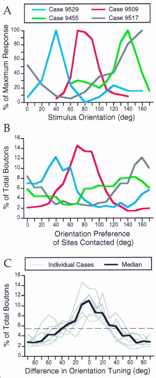
Correspondence between orientation tuning of injection sites and specificity of bouton distributions for four cases.A, Orientation tuning curves determined from recordings of multiunit activity that were made through the biocytin-filled pipettes at each injection site. Normalized responses are plotted versus stimulus orientation. B, Bouton tuning curves for the same cases shown in A, plotted in the same color as_A_. For each case, the percentage of the total number of boutons that overlie sites with a given orientation preference is plotted. Only boutons found at distances >500 μm from the injection site were used in this analysis. Each curve has a peak at or near the peak of the physiologically determined tuning curve shown in_A_. C, Data from all seven of our combined imaging and biocytin injection experiments. The bouton tuning curves for each case are expressed as the percentage of the boutons that contact sites that differ in orientation preference from the injection site by a specified amount. Individual cases are shown in_gray_, and the median is shown in black. The dashed line shown at 5.56% reflects the percentage of boutons expected in each of the 18 bins if the boutons were distributed evenly over the map of orientation preference.
Axial specificity of horizontal connections
Before describing our analysis of axial specificity of horizontal connections it is necessary to describe the organization of the map of visual space in tree shrew V1. As illustrated in Figure7A, the tree shrew has a well developed striate cortex with a prominent V1/V2 border that is clearly discerned in Nissl-stained sections. An earlier physiological study by Kaas et al. (1972) demonstrated that, as in other species, the V1/V2 border corresponds to the representation of the vertical meridian in visual space. The horizontal meridian, as well as other iso-elevation lines, intersects this border at approximately right angles (Kaas, 1980).
Fig. 7.
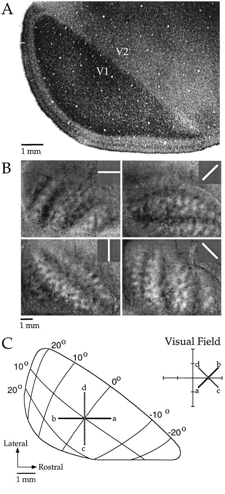
The map of visual space in tree shrew V1.A, Photomicrograph of a Nissl-stained section of visual cortex. V1 stands out clearly as the darkly stained_region of the section. B, Topographic difference images for four stimulus angles. The dark bands and_light bands ∼0.5–1.0 mm wide in each image reflect areas of cortex that were differentially activated by the two grating patterns for that stimulus angle (see Materials and Methods for details). The distance between a pair of dark or light bands corresponds to 10° in the map of visual space. The 0° and 90° images represent iso-elevation and iso-azimuth lines. C, Diagram of the right visual field and left visual cortex of the tree shrew, modified from a figure by Kaas (1980). Lines at 45° orientation (black line) and at 135° orientation (gray line) are shown as they would appear in the visual field and in the cortex.
To confirm the geometry of the map of visual space, we used optical imaging with a stimulation paradigm similar to one developed byCampbell and Blasdel (1995). The technique uses difference imaging for spatial location with two gratings of the same orientation to identify areas of cortex that respond preferentially to stimulation of a particular line in visual space (see Methods for details). Data obtained from one animal using this technique to visualize 0°, 45°, 90°, and 135° lines in the map of visual space are shown in Figure8B. Similar results were obtained in two other animals. Results from these experiments were in general agreement with earlier mapping studies (Kaas et al., 1972; Kaas, 1980). The map of visual space presented in Figure 7C has been slightly modified from one originally presented by Kaas (1980) to reflect the geometry and spacing of iso-azimuth and iso-elevation lines as measured by optical imaging.
Fig. 8.

Bouton distributions from four cases. The preferred orientation for each case is shown in the top right of each panel. The axis in cortex corresponding to the preferred orientation is indicated by the _gray rectangle_underlying each distribution. Each point indicates an individual bouton. Note the dense distribution of boutons found near the injection site and more patchy distribution found at longer distances. In each case, the distribution is elongated along an axis that corresponds to the preferred orientation of the injection site.
Figure 7, B and C, confirms that the map of visual space is largely isotropic near the center of V1, and all of our injections were placed in this area. In addition, they illustrate that it is possible to specify the axis in cortex that corresponds to a particular axis in the visual field by simply rotating the appropriate number of degrees from the V1/V2 border axis. For example, Figure7C depicts a 45° axis (black lines) and 135° axis (gray lines) as they would appear in both the right visual field and the left visual cortex. Thus, the presence of a prominent V1/V2 border and the lack of large distortions in the map of visual space greatly facilitate the examination of axial specificity of horizontal connections in the tree shrew.
As described in other species, injections of biocytin into layer 2/3 resulted in a distribution of labeled terminals that was elongated across the cortical surface. The axis of elongation was found to vary from case to case and was systematically related to the orientation preference of the injection site. This basic relationship can be appreciated by examining the distribution of labeled terminals compared to an outline of V1 as is done for four cases in Figure 8. In each panel, the axis of elongation of the labeled terminals can be compared to the V1/V2 border (vertical meridian). As illustrated in Figure8A, an injection into a site with a preferred orientation near vertical resulted in a distribution of labeled terminals that was elongated parallel to the V1/V2 border. In contrast, an injection into a site with a preferred orientation of near horizontal (Fig. 8C) resulted in a distribution that was elongated perpendicular to the V1/V2 border. In each of the cases that we examined, we found a similar relationship: layer 2/3 neurons give rise to horizontal connections that extend for longer distances, and give rise to more boutons, along an axis of the visual field map that corresponds to their preferred stimulus orientation.
Quantification of the systematic relationship between the axis of elongation of the terminal distributions and the preferred stimulus orientation of the biocytin injection sites is illustrated in Figures9, 10, 11. The polar plots in Figure 9 illustrate the number of labeled terminals found in successive 10° sectors surrounding an injection site for the same four cases shown in Figure 8. In these plots, the distance of each point from the center of the circle indicates the relative number of boutons found in that 10° sector. The 0° sector for each polar plot was assigned by drawing a line through the center of the injection site orthogonal to the V1/V2 border. Sectors were then assigned in a clockwise manner, resulting in the 90° sector corresponding to an axis that is parallel to the V1/V2 border. With this reference scheme, the distribution of labeled terminals across the visual field map can be compared directly to the preferred stimulus orientation recorded from the units at the injection site (shown to the upper right of each plot). In each case, the dominant axis of the terminal polar plot matches the preferred stimulus orientation recorded from the site before the injection.
Fig. 9.

Quantification of bouton distributions for four cases. For each case, the number of boutons found in successive 10° sectors around the injection is quantified. Distance from the origin indicates the number of boutons found in a given sector normalized to the maximum number of boutons found in any sector for that case. The 0° sector was assigned by drawing a line through the injection site that was orthogonal to the V1/V2 border, and the remaining sectors were assigned in clockwise manner. Only boutons outside of 500 μm were used in this analysis. The preferred orientation of the injection site for each case is indicated by the black bar in each_inset_. The thin gray line in the visual field diagrams and the gray dashed lines in the polar plots correspond to the vertical meridian.
Fig. 10.
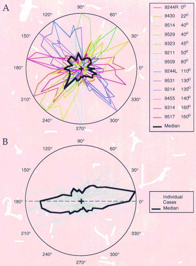
Correspondence between preferred orientation of injection sites and the axial specificity of the bouton distributions.A, Polar plots are shown for all 13 cases examined for axial specificity. Each polar plot was constructed as described in Figure 9 and is color-coded according to the orientation preference of the injection site for that case. The black curve is the median of the 13 cases. B, Data from all 13 cases were combined by rotating each curve by a number of degrees equal to the orientation preference at the injection site for that case. Gray lines indicate individual cases, and the _black line_indicates the normalized median of all 13 cases.
Fig. 11.
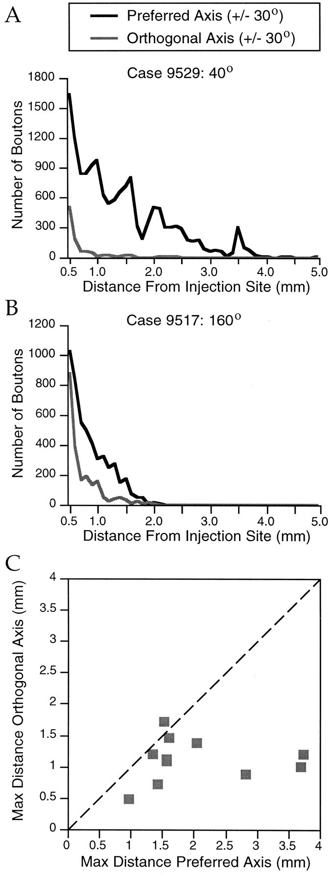
Quantification of elongation of bouton distributions. A, Number of boutons versus distance in 100 μm bins along both the preferred (black curve) and orthogonal (gray curve) axes (±30°). Preferred orientation for this case was 40°. B, Same information shown for a case that had a preferred orientation of 160°.C, Scatterplot showing the maximum distance at which boutons were found to exceed a minimum density of 40 boutons/0.01 mm2 along the preferred and orthogonal axes (±30°) for 10 cases. Dashed lines indicate equal distance along preferred and orthogonal axes.
Our sample of injection sites from 13 cases included a wide range of preferred stimulus orientations, and for each orientation we found a corresponding bias in the axial distribution of labeled terminals. Figure 10A shows the terminal polar plots for all 13 of our cases and illustrates that each injection resulted in a distribution with a distinct axial bias. The degree to which the variation among cases in the axial alignment of terminal distributions is a function of the preferred stimulus orientation of the injection site is illustrated in Figure 10B. In this figure, the terminal polar plots have been aligned by rotating them by an angle that corresponds to the difference between the preferred stimulus orientation of the injection site and horizontal (0°). For example, the bouton distribution for a site with a preferred stimulus orientation of 22° was rotated clockwise by 22°. Individual profiles are illustrated by the gray curves and the black curve represents the median for all of the cases examined. On average, neurons in layer 2/3 give rise to four times as many terminals along an axis that corresponds to their preferred stimulus orientation (±35°) than along the orthogonal axis (±35°).
The axial bias in the distribution of connections is reflected not only in the number of labeled terminals, but in the distance of the labeled terminals from the injection site. Labeled boutons were consistently found to extend greater distances from the injection site along the axis of the visual field map that corresponds to their preferred stimulus orientation. This feature of the bouton distributions is illustrated for two cases in Figure 11, A and B, that plot the number of boutons versus distance along either the preferred or orthogonal axes. To further quantify this relationship we determined the maximum distance along the preferred and orthogonal axes (±30°) at which a minimum density of 40 boutons/0.01 mm2was exceeded for each case. For the case shown in Figure11A, the maximum extension along the preferred axis was 3.73 mm and the maximum extension along the orthogonal axis was 0.96 mm. This information is shown for all 10 cases for which the required data were available in Figure 11C. The maximum distance at which boutons were found along the preferred axis (median 1.77 mm) was significantly different from the maximum distance along the orthogonal axis (median 1.16 mm; p < 0.004, Wilcoxon signed rank test).
DISCUSSION
The results of this study confirm the results of previous studies in cats and monkeys showing that long-range horizontal connections selectively link patches of neurons that have similar orientation preferences (Gilbert and Wiesel, 1989; Blasdel et al., 1992; Malach et al., 1993). In addition, our results reveal a new feature of long-range horizontal connections that has not been described before: orientation-specific anisotropy. Horizontal connections in the tree shrew extend for greater distances and distribute more terminal boutons along an axis of the visual field map that corresponds to the preferred orientation of the injection site. In the next sections we relate these results to those of previous studies and consider the implications of modular and axial specificity for understanding the function of horizontal connections.
Modular specificity of local and long-distance horizontal connections
Our results demonstrate that long-distance horizontal connections in V1 have a strong bias toward connecting regions with similar orientation preferences, and a degree of specificity that is commensurate with the orientation tuning of the neurons they interconnect. In several cases, for example, bouton tuning curves, constructed from an analysis of the position of boutons relative to the orientation map, were remarkably similar in both their peak and half-width to the physiologically defined orientation tuning curves for multi-unit activity at the injection site (compare tuning curves in Fig. 6A, B). In addition, the peak of the median bouton tuning curve constructed from all of the cases was centered on the preferred orientation of the injection site and 57.6% of the labeled boutons contacted sites with a preferred orientation that was within 35° of the peak. This degree of specificity is comparable to that reported for long-range horizontal connections in macaque V1 (Malach et al., 1993).
Although, for technical reasons, it proved more difficult to characterize the orientation specificity of boutons located within 500 μm of the injection site, on the whole, these local connections appear less specific than their long-distance counterparts. In many cases, for example, a nearly uniform halo of labeled terminals surrounded the biocytin injection site and the tuning curves for the local bouton distribution were correspondingly flat. Because we did not plot boutons inside the area of the injection site that contained labeled cell bodies and dendrites, it is likely that we have underestimated the degree of iso-orientation connectivity of local connections. Nevertheless, unlike long-range connections, labeled terminals near the injection site are located in regions of the orientation preference map that include the full range of values. Observations from macaque visual cortex also suggest a lower specificity for local horizontal connections (Amir et al., 1993; Malach et al., 1993).
The difference in specificity of local and long-distance connections could reflect a difference in the relative contribution of excitatory and inhibitory neurons. Previous studies have shown that, compared to excitatory connections, inhibitory connections in layer 2/3 extend for shorter distances (Albus et al., 1991; Matsubara and Boyd, 1992; Albus and Wahle, 1994), are less specific for orientation domains (Kisvarday and Eysel, 1993; Kisvarday et al., 1994;), and tend to be more uniformly distributed around the injection site (Albus et al., 1991;Matsubara and Boyd, 1992; Albus and Wahle, 1994). Thus, it is possible that the distribution of boutons that we observe results from a nonspecific ring of connections contributed by GABAergic neurons that is superimposed upon the more specific connections established by pyramidal neurons. Clearly, determining the actual contribution of these two classes of neurons to the pattern of local connections will require an analysis at the single cell level.
Axial specificity of horizontal connections
This is the first demonstration of an anisotropy in horizontal connections which varies from site to site and is systematically related to the orientation selective responses of cortical neurons. Previous studies in visual cortex of cats and macaque monkeys have noted that horizontal connections tend to form distributions that are elongated along a particular axis, and in some cases the observed anisotropy in horizontal connections was explained in terms of a corresponding anisotropy in the map of visual space (McGuire et al., 1991; Yoshioka et al., 1992; Amir et al., 1993; Malach et al., 1993;Grinvald et al., 1994). These authors reported that horizontal connections appear to consistently extend for longer distances along the vertical axis of the map of visual space, corresponding to the fact that cortical magnification factor (amount of cortical surface area per unit visual space) is greatest along this axis. However, other investigators have reported elongated distributions which could not be explained by the anisotropy in the map of visual space (Gilbert and Wiesel, 1983, 1989; Kisvarday and Eysel, 1992). Thus, the exact extent to which anisotropies in the map of visual space, or other factors, determine the distribution of horizontal connections has remained unclear.
A global feature like magnification factor cannot explain the consistent relationship between orientation preference and axis of elongation in the tree shrew. Nevertheless, it might account for some of the variability that we observed in the absolute amount of elongation along the preferred axis. For example, some of the most elongated distributions in the tree shrew had axes that ran parallel to the V1/V2 border, whereas some of the least elongated ran perpendicular to the border. We did not observe a consistent relation between map anisotropy and degree of elongation, but this relationship might have been obscured by other factors such as the size and placement of the injection site, or variations in the quality of biocytin uptake and transport.
An axial alignment of horizontal connections related to orientation preference was first suggested by Mitchison and Crick (1982) as an explanation for the observation that injections of tracers in V1 produce patchy labeling, even when the injection is large enough to involve sites with a wide range of orientation preferences. Using computer simulations, they showed that if the network of horizontal connections was constrained by just one rule of “like connects to like” then a continuous distribution of label would result from a large injection. On the other hand, if two rules requiring axial and modular specificity of horizontal connections were used to model horizontal connectivity, then a patchy distribution of label would result from a large injection. The demonstration of combined modular and axial specificity in the tree shrew, and the observation of patchy distributions of labeled neurons after large tracer injections in V1 of many species, suggests that modular specificity alone might be insufficient to explain the distribution of horizontal connections. Indeed, preliminary results, using combined optical imaging and biocytin injections, suggest that a combined modular and axial specificity might be present in the squirrel monkey (Sincich and Blasdel, 1995). It is possible that a relationship between preferred orientation and axis of projection also exists in cats and other primates but is difficult to demonstrate due to other factors such as large anisotropies in the map of visual space.
Functional implications
Combined with the evidence that horizontal connections are largely reciprocal (Kisvarday and Eysel, 1992), these results indicate that individual neurons in layer 2/3 receive input from other neurons whose receptive fields are co-oriented (of similar orientation preference) and co-axial (displaced along an axis in visual space that corresponds to their preferred orientation; Fig.12A,B). This relationship raises the possibility that horizontal connections might contribute to the orientation selectivity of layer 2/3 neurons. For example, a neuron that responds best to a vertical stimulus might do so, at least in part, because it receives input from a network of other layer 2/3 neurons whose receptive fields are aligned along the vertical axis of visual space. This arrangement could be viewed as the intracortical equivalent of the Hubel and Wiesel model in which layer 4 neurons derive their orientation selectivity by sampling from a population of lateral geniculate nucleus neurons whose receptive fields are aligned along an axis in visual space (Hubel and Wiesel, 1962). Presumably, the intrinsic circuitry in layer 2/3 acts in concert with orientation selective inputs derived from layer 4 to generate the orientation selectivity of layer 2/3 neurons. Indeed, the contribution of axially aligned horizontal connections could explain why layer 2/3 neurons in the tree shrew and ferret are more tightly tuned for orientation than those in layer 4 (Humphrey et al., 1980a; Chapman and Stryker, 1993). It could also explain why many neurons exhibit sharper orientation tuning (a smaller half width at half height) when longer stimuli are used to determine tuning (Henry et al., 1974).
Fig. 12.

Summary of specificity of horizontal connections in V1. A, Example of axon arborizations from two cells shown over a combined map of visual space and difference map of orientation preference. The dark regions of the difference map indicate regions that prefer 90°, and the_lighter areas_ indicate areas that prefer 0°. A neuron found in a dark region of the map projects to other areas of the map with the same orientation preference and that lie along a line corresponding to a vertical line in the map of visual space. A neuron found in a light region of the map (orientation preference 0°) projects to other parts of the cortex that prefer 0° and that lie along a horizontal line in the map of visual space. B, Input to layer 2/3 cells via horizontal connections. Because horizontal connections are largely reciprocal, cells in layer 2/3 will receive input from other layer 2/3 cells with the same orientation preference, the receptive fields of which are displaced along a line in visual space. The solid rectangles indicate the receptive fields of the two cells shown in A. The open rectangles indicate the receptive fields of cells that would provide input to these two cells via horizontal connections. Nearby cells with overlapping receptive fields are omitted for clarity.
Because of their extensive spread, horizontal connections have been implicated as one of the potential substrates for receptive field surround effects—changes in the response pattern of neurons produced by visual stimulation of the region that lies outside of the receptive field as defined by a small, simple stimulus (for review, see Gilbert, 1992). In the tree shrew, for example, these connections extend for up to 4 mm from the injection site—a distance that corresponds to ∼20° of visual space—whereas the classically defined receptive field at this eccentricity extends for less than 5°. The results of the present study suggest that horizontal connections could be the source of a particular class of receptive field surround effects that exhibit axial specificity, exerting a greater influence in regions of visual space that lie along the axis of the neuron’s preferred orientation (i.e., end-zones) than along the orthogonal axis (side-zones). Effects of this type have been described in both cat and monkey striate cortex and in several cases the effects are primarily facilitatory (Nelson and Frost, 1985; Fiorani et al., 1992; Kapadia, 1995). Some neurons in macaque visual cortex, for example, show an enhanced response to placement of an additional stimulus outside the receptive field (Kapadia et al., 1995); this enhancement occurs only when the additional element is at the preferred orientation and collinear with the stimulus placed in the receptive field. Neurons in layer 2/3 of tree shrew striate cortex also exhibit long range axially specific facilitatory effects. For example, many layer 2/3 neurons in the tree shrew exhibit length summation, showing an increase in response with increasing stimulus length for stimuli as long as 40°. In addition, stimulation of the end-zones alone, without stimulation of the classical receptive field, is sufficient to drive some layer 2/3 neurons, whereas stimulation of the side-zones is ineffective (Bosking and Fitzpatrick, 1995).
Long-range collinear facilitatory effects could serve as one of the important mechanisms that underlies the perception of continuity in visual patterns. Indeed, the perception of continuity appears to depend critically on the very features that characterize long-range horizontal connections. For example, the ability of human observers to detect contours composed of small oriented line segments from among an array of distracter elements is dependent upon both the orientation and position of the elements (Field et al., 1993). Observers are much better at detecting a contour composed of multiple segments when the segments are aligned with the path of the contour than when they are aligned orthogonal to the path. Similarly, detection of an oriented line segment or a grating is enhanced by flanking the stimulus with other collinear stimuli (Polat and Sagi, 1993; Kapadia et al., 1995).
Thus, the modular and axial specificity of horizontal connections seems well suited for supporting the perception of contours, especially under noisy or degraded stimulus conditions.
Footnotes
This work was supported by National Eye Institute Grant EY06821. We thank Martha Foster for expert assistance with histology and plotting of bouton data, Mike Weliky for assistance with software, and Len White, Michele Pucak, and Justin Crowley for comments on this manuscript.
Correspondence should be addressed to William H. Bosking, Box 3209, Department of Neurobiology, Duke University Medical Center, Durham, NC 27710.
REFERENCES
- 1.Albus K, Wahle P. The topography of tangential inhibitory connections in the postnatally developing and mature striate cortex of the cat. Eur J Neurosci. 1994;6:779–792. doi: 10.1111/j.1460-9568.1994.tb00989.x. [DOI] [PubMed] [Google Scholar]
- 2.Albus K, Wahle P, Lubke J, Matute C. The contribution of GABA-ergic neurons to horizontal intrinsic connections in upper layers of the cat’s striate cortex. Exp Brain Res. 1991;85:235–239. doi: 10.1007/BF00230006. [DOI] [PubMed] [Google Scholar]
- 3.Amir Y, Harel M, Malach R. Cortical hierarchy reflected in the organization of intrinsic connections in macaque monkey visual cortex. J Comp Neurol. 1993;334:19–46. doi: 10.1002/cne.903340103. [DOI] [PubMed] [Google Scholar]
- 4.Blasdel GG. Orientation selectivity, preference, and continuity in monkey striate cortex. J Neurosci. 1992;12:3139–3161. doi: 10.1523/JNEUROSCI.12-08-03139.1992. [DOI] [PMC free article] [PubMed] [Google Scholar]
- 5.Blasdel GG, Yoshioka T, Levitt JB, Lund JS. Correlation between patterns of lateral connectivity and patterns of orientation preference in monkey striate cortex. Soc Neurosci Abstr. 1992;18:389. [Google Scholar]
- 6.Bolz J, Gilbert CD. The role of horizontal connections in generating long receptive fields in the cat visual cortex. Eur J Neurosci. 1989;1:263–268. doi: 10.1111/j.1460-9568.1989.tb00794.x. [DOI] [PubMed] [Google Scholar]
- 7.Bonhoeffer T, Grinvald A. Iso-orientation domains in cat visual cortex are arranged in pinwheel-like patterns. Nature. 1991;353:429–431. doi: 10.1038/353429a0. [DOI] [PubMed] [Google Scholar]
- 8.Bonhoeffer T, Grinvald A. The layout of iso-orientation domains in area 18 of cat visual cortex: optical imaging reveals a pinwheel-like organization. J Neurosci. 1993;13:4157–4180. doi: 10.1523/JNEUROSCI.13-10-04157.1993. [DOI] [PMC free article] [PubMed] [Google Scholar]
- 9.Bosking WH, Fitzpatrick D. Physiological correlates of anisotropy in horizontal connections: length summation properties of neurons in layers 2 and 3 of tree shrew striate cortex. Soc Neurosci Abstr. 1995;21:1751. [Google Scholar]
- 10.Campbell D, Blasdel GG. Optical measurement of cortical magnification factors in new and old world primates. Soc Neurosci Abstr. 1995;21:771. [Google Scholar]
- 11.Chapman B, Stryker MP. Development of orientation selectivity in ferret visual cortex and effects of deprivation. J Neurosci. 1993;13:5251–5262. doi: 10.1523/JNEUROSCI.13-12-05251.1993. [DOI] [PMC free article] [PubMed] [Google Scholar]
- 12.Field DJ, Hayes A, Hess RF (1993) Contour integration by the human visual system: evidence for a local “association field.” Vision Res 33:173–193. [DOI] [PubMed]
- 13.Fiorani M, Rosa MGP, Gattass R, Rocha-Miranda CE. Dynamic surrounds of receptive fields in primate striate cortex: a physiological basis for perceptual completion? Proc Natl Acad Sci USA. 1992;89:8547–8551. doi: 10.1073/pnas.89.18.8547. [DOI] [PMC free article] [PubMed] [Google Scholar]
- 14.Gilbert CD. Horizontal integration and cortical dynamics. Neuron. 1992;9:1–13. doi: 10.1016/0896-6273(92)90215-y. [DOI] [PubMed] [Google Scholar]
- 15.Gilbert CD, Wiesel TN. Morphology and intracortical projections of functionally characterised neurones in the cat visual cortex. Nature. 1979;280:120–125. doi: 10.1038/280120a0. [DOI] [PubMed] [Google Scholar]
- 16.Gilbert CD, Wiesel TN. Clustered intrinsic connections in cat visual cortex. J Neurosci. 1983;3:1116–1133. doi: 10.1523/JNEUROSCI.03-05-01116.1983. [DOI] [PMC free article] [PubMed] [Google Scholar]
- 17.Gilbert CD, Wiesel TN. Columnar specificity of intrinsic horizontal and corticocortical connections in cat visual cortex. J Neurosci. 1989;9:2432–2442. doi: 10.1523/JNEUROSCI.09-07-02432.1989. [DOI] [PMC free article] [PubMed] [Google Scholar]
- 18.Grinvald A, Lieke EE, Frostig RD, Gilbert CD, Wiesel TN. Functional architecture of cortex revealed by optical imaging of intrinsic signals. Nature. 1986;324:361–364. doi: 10.1038/324361a0. [DOI] [PubMed] [Google Scholar]
- 19.Grinvald A, Lieke EE, Frostig RD, Hildesheim R. Cortical point-spread function and long-range lateral interactions revealed by real-time optical imaging of Macaque monkey primary visual cortex. J Neurosci. 1994;14:2545–2568. doi: 10.1523/JNEUROSCI.14-05-02545.1994. [DOI] [PMC free article] [PubMed] [Google Scholar]
- 20.Henry GH, Dreher B, Bishop PO. Orientation specificity of cells in cat striate cortex. J Neurophysiol. 1974;37:1394–1409. doi: 10.1152/jn.1974.37.6.1394. [DOI] [PubMed] [Google Scholar]
- 21.Hubel DH, Wiesel TN. Receptive fields, binocular interaction and functional architecture in the cat’s visual cortex. J Physiol (Lond) 1962;160:106–154. doi: 10.1113/jphysiol.1962.sp006837. [DOI] [PMC free article] [PubMed] [Google Scholar]
- 22.Humphrey AL, Skeen LC, Norton TT. Topographic organization of the orientation column system in the striate cortex of the tree shrew (Tupaia glis). I. Microelectrode recording. J Comp Neurol. 1980a;192:531–543. doi: 10.1002/cne.901920311. [DOI] [PubMed] [Google Scholar]
- 23.Humphrey AL, Skeen LC, Norton TT. Topographic organization of the orientation column system in the striate cortex of the tree shrew (Tupaia glis). II. Deoxyglucose mapping. J Comp Neurol. 1980b;192:544–566. doi: 10.1002/cne.901920312. [DOI] [PubMed] [Google Scholar]
- 24.Kaas JH. A comparative survey of visual cortex organization in mammals. In: Ebbesson SOE, editor. Comparative neurology of the telencephalon. Plenum; New York: 1980. pp. 483–502. [Google Scholar]
- 25.Kaas JH, Hall WC, Killackey H, Diamond IT. Visual cortex of the tree shrew (Tupaia glis): architectonic subdivisions and representations of the visual field. Brain Res. 1972;42:491–496. doi: 10.1016/0006-8993(72)90548-3. [DOI] [PubMed] [Google Scholar]
- 26.Kapadia MK, Ito M, Gilbert CD, Westheimer G. Improvement in visual sensitivity by changes in local context: parallel studies in human observers and in V1 of alert monkeys. Neuron. 1995;15:843–856. doi: 10.1016/0896-6273(95)90175-2. [DOI] [PubMed] [Google Scholar]
- 27.Kisvarday ZF, Eysel UT. Cellular organization of reciprocal patchy networks in layer III of cat visual cortex (area 17). Neuroscience. 1992;46:275–286. doi: 10.1016/0306-4522(92)90050-c. [DOI] [PubMed] [Google Scholar]
- 28.Kisvarday ZF, Eysel UT. Functional and structural topography of horizontal inhibitory connections in cat visual cortex. Eur J Neurosci. 1993;5:1558–1572. doi: 10.1111/j.1460-9568.1993.tb00226.x. [DOI] [PubMed] [Google Scholar]
- 29.Kisvarday ZF, Kim DS, Eysel UT, Bonhoeffer T. Relationship between lateral inhibitory connections and the topography of the orientation map in cat visual cortex. Eur J Neurosci. 1994;6:1619–1632. doi: 10.1111/j.1460-9568.1994.tb00553.x. [DOI] [PubMed] [Google Scholar]
- 30.Livingstone MS, Hubel DH. Specificity of intrinsic connections in primate primary visual cortex. J Neurosci. 1984;4:2830–2835. doi: 10.1523/JNEUROSCI.04-11-02830.1984. [DOI] [PMC free article] [PubMed] [Google Scholar]
- 31.Malach R, Amir Y, Harel M, Grinvald A. Relationship between intrinsic connections and functional architecture revealed by optical imaging and in vivo targeted biocytin injections in primate striate cortex. Proc Natl Acad Sci USA. 1993;90:10469–10473. doi: 10.1073/pnas.90.22.10469. [DOI] [PMC free article] [PubMed] [Google Scholar]
- 32.Matsubara JA, Boyd JD. Presence of GABA-immunoreactive neurons within intracortical patches in area 18 of the cat. Brain Res. 1992;583:161–170. doi: 10.1016/s0006-8993(10)80020-4. [DOI] [PubMed] [Google Scholar]
- 33.Matsubara JA, Cynader MS, Swindale NV, Stryker MP. Intrinsic projections within visual cortex: evidence for orientation specific local connections. Proc Natl Acad Sci USA. 1985;82:935–939. doi: 10.1073/pnas.82.3.935. [DOI] [PMC free article] [PubMed] [Google Scholar]
- 34.Matsubara JA, Cynader MS, Swindale NV. Anatomical properties and physiological correlates of the intrinsic connections in cat area 18. J Neurosci. 1987;7:1428–1446. doi: 10.1523/JNEUROSCI.07-05-01428.1987. [DOI] [PMC free article] [PubMed] [Google Scholar]
- 35.McGuire BA, Gilbert CD, Rivlin PK, Wiesel TN. Targets of horizontal connections in macaque primary visual cortex. J Comp Neurol. 1991;305:370–392. doi: 10.1002/cne.903050303. [DOI] [PubMed] [Google Scholar]
- 36.Mitchison G, Crick F. Long axons within the striate cortex: their distribution, orientation, and patterns of connection. Proc Natl Acad Sci USA. 1982;79:3661–3665. doi: 10.1073/pnas.79.11.3661. [DOI] [PMC free article] [PubMed] [Google Scholar]
- 37.Nelson JI, Frost BJ. Intracortical facilitation among co-oriented, co-axially aligned simple cells in cat striate cortex. Exp Brain Res. 1985;61:54–61. doi: 10.1007/BF00235620. [DOI] [PubMed] [Google Scholar]
- 38.Obermayer K, Blasdel GG. Geometry of orientation and ocular dominance columns in monkey striate cortex. J Neurosci. 1993;13:4114–4129. doi: 10.1523/JNEUROSCI.13-10-04114.1993. [DOI] [PMC free article] [PubMed] [Google Scholar]
- 39.Polat U, Sagi D. Lateral interactions between spatial channels: suppression and facilitation revealed by lateral masking experiments. Vision Res. 1993;33:993–999. doi: 10.1016/0042-6989(93)90081-7. [DOI] [PubMed] [Google Scholar]
- 40.Rockland KS, Lund JS. Widespread periodic intrinsic connections in the tree shrew visual cortex. Science. 1982;215:1532–1534. doi: 10.1126/science.7063863. [DOI] [PubMed] [Google Scholar]
- 41.Sincich L, Blasdel GG. Lateral connections and orientation pref-erence in layers II/III of squirrel monkey striate cortex. Soc Neurosci Abstr. 1995;21:393. [Google Scholar]
- 42.T’so DY, Gilbert CD, Wiesel TN. Relationships between horizontal interactions and functional architecture in cat striate cortex as revealed by cross-correlation analysis. J Neurosci. 1986;6:1160–1170. doi: 10.1523/JNEUROSCI.06-04-01160.1986. [DOI] [PMC free article] [PubMed] [Google Scholar]
- 43.Usrey WM, Fitzpatrick D. Specificity in the axonal connections of layer VI neurons in tree shrew striate cortex: evidence for distinct granular and supragranular systems. J Neurosci. 1996;16:1203–1218. doi: 10.1523/JNEUROSCI.16-03-01203.1996. [DOI] [PMC free article] [PubMed] [Google Scholar]
- 44.Weliky M, Kandler K, Fitzpatrick D, Katz LC. Patterns of excitation and inhibition evoked by horizontal connections in visual cortex share a common relationship to orientation columns. Neuron. 1995;15:541–552. doi: 10.1016/0896-6273(95)90143-4. [DOI] [PubMed] [Google Scholar]
- 45.Yoshioka T, Blasdel GG, Levitt JB, Lund JS. Patterns of lateral connections in macaque visual area V1 revealed by biocytin histochemistry and functional imaging. Soc Neurosci Abstr. 1992;18:299. [Google Scholar]