Temporal Dynamics of Graded Synaptic Transmission in the Lobster Stomatogastric Ganglion (original) (raw)
Abstract
Synaptic transmission between neurons in the stomatogastric ganglion of the lobster Panulirus interruptus is a graded function of membrane potential, with a threshold for transmitter release in the range of −50 to −60 mV. We studied the dynamics of graded transmission between the lateral pyloric (LP) neuron and the pyloric dilator (PD) neurons after blocking action potential-mediated transmission with 0.1 μm tetrodotoxin. We compared the graded IPSPs (gIPSPs) from LP to PD neurons evoked by square pulse presynaptic depolarizations with those potentials evoked by realistic presynaptic waveforms of variable frequency, amplitude, and duty cycle. The gIPSP shows frequency-dependent synaptic depression. The recovery from depression is slow, and as a result, the gIPSP is depressed at normal pyloric network frequencies. Changes in the duration of the presynaptic depolarization produce nonintuitive changes in the amplitude and time course of the postsynaptic responses, which are again frequency-dependent. Taken together, these data demonstrate that the measurements of synaptic efficacy that are used to understand neural network function are best made using presynaptic waveforms and patterns of activity that mimic those in the functional network.
Keywords: graded synaptic transmission, pyloric network, central pattern generation, oscillations, synaptic depression, inhibition
Most rhythmic movements are produced by central pattern-generating circuits (Marder and Calabrese, 1996). In many cases, the rhythmic movements are produced over a significant frequency range without appreciable alteration of the fundamental phase relationships or the character of the movement; e.g., an animal is allowed to breathe or to walk at different rates, slowly or quickly. Because circuit dynamics depend on both synaptic and intrinsic properties, it is interesting to ask how these dynamics are affected by changes in network frequency. In this paper we present the effects of frequency on the graded synaptic transmission between neurons of the pyloric circuit of the spiny lobster Panulirus interruptus.
The pyloric network of the stomatogastric ganglion (STG) of P. interruptus is one of the best understood pattern-generating circuits. The connectivity among these neurons and their intrinsic membrane properties have been determined (Selverston and Miller, 1980;Eisen and Marder, 1982; Miller and Selverston, 1982a,b). Both in vivo and in vitro studies in a variety of crustacean species have shown that the triphasic pyloric rhythm operates over a frequency range from ∼0.1 to ∼2.5 Hz (Ayers and Selverston, 1979;Rezer and Moulins, 1983; Eisen and Marder, 1984; Turrigiano and Heinzel, 1992; Hooper, 1997a,b). One of the essential puzzles is how the pyloric rhythm can produce approximately the same motor pattern over such a wide frequency range. One possibility is that time-dependent changes in functional synaptic strength, such as facilitation and depression, play a critical role in maintaining network phase relationships as the frequency changes. This theory prompted us to examine the dynamics of graded synaptic transmission at one of the synaptic connections that is important for frequency regulation of the pyloric rhythm.
The chemical synaptic connections between STG neurons are inhibitory (Maynard, 1972; Mulloney and Selverston, 1974a,b). The threshold for transmitter release is close to the resting potential, and synaptic release is both spike-mediated and graded (Maynard and Walton, 1975;Graubard, 1978; Graubard et al., 1980, 1983; Johnson and Harris-Warrick, 1990; Johnson et al., 1995). At some synapses the graded component of transmitter release is significantly larger than that evoked by action potentials and is the major contributor to network dynamics (Raper, 1979; Graubard et al., 1983; Hartline et al., 1988). When spike-mediated transmission is blocked by tetrodotoxin (TTX), an alternating pattern of slow wave oscillation characteristic of the pyloric rhythm can be generated by applying various activating modulatory substances (Raper, 1979; Anderson and Barker, 1981).
Graded synaptic transmission between pyloric neurons has been extensively studied in a “static” context in which the time dependence of the transmission was ignored (Graubard, 1978; Graubard et al., 1980, 1983; Johnson and Harris-Warrick, 1990; Johnson et al., 1995). However, graded synaptic transmission between pyloric neurons shows depression and depends on the amplitude, frequency, and shape of the depolarization of the presynaptic neuron (Graubard et al., 1989;Hartline and Graubard, 1992). Here we give, for the first time, a detailed characterization of the dynamics of graded inhibitory transmission from the lateral pyloric (LP) neuron to the two pyloric dilator (PD) neurons. These synapses are the sole feedback from the pyloric constrictors to the pyloric pacemaker group [consisting of the anterior burster (AB) neuron and the two PD neurons]. This analysis provides some counterintuitive results that may help us to understand how frequency and duty cycle-dependent changes in synaptic strength participate in maintaining a constant pyloric rhythm over a wide frequency range.
MATERIALS AND METHODS
All experiments were performed on the spiny lobster P. interruptus. The experiments reported in this paper used 17 animals, both male and female. Animals weighed between 400 and 800 gm. Animals were obtained from Don Tomlinson (San Diego, CA) and were maintained in artificial seawater tanks at 12–15°C up to several weeks before use.
Standard procedures (Selverston et al., 1976; Harris-Warrick et al., 1992) were used to isolate the complete stomatogastric nervous system (the STG attached to the esophageal and paired commissural ganglia). The preparations were superfused during the dissection with cool, 13–15°C, pH 7.4–7.5, normal saline containing (in mm): 479 NaCl, 13.7 KCl, 3.9 NaSO4, 10 MgSO4, 2 glucose, and 5.1 Trizma base acid.
Microelectrodes were pulled on a Flaming–Brown horizontal puller and were filled with 2 m KCl. The electrode resistances were 8–12 MΩ. All neurons were identified by their stereotypical axonal projections in identified nerves using conventional techniques (Selverston et al., 1976; Harris-Warrick et al., 1992).
The presynaptic (LP) cell was impaled with two electrodes, and each postsynaptic (PD) cell was impaled with one electrode. After identification of these neurons, the preparation was superfused with 0.1 μm TTX to block action potentials and to eliminate pyloric slow wave oscillation. The preparation was then kept at room temperature (21°C) to increase the amplitude of the graded IPSP (gIPSP) (Johnson et al., 1991). This temperature is within the normal range of water temperatures in these animals’ natural habitat. The presynaptic cell was voltage-clamped with an Axoclamp 2A amplifier (Axon Instruments) in the two-electrode voltage-clamp mode. Postsynaptic cells were recorded in current-clamp mode. The postsynaptic membrane potential was depolarized by current injection (see the legends of individual figures) to keep this potential far from the reversal potential of the synapse (approximately −70 mV), thus ensuring that the gIPSPs were large in amplitude. An AT-MIO-16E-2 board was used both for data acquisition and for current injection with LabWindows/CVI software (National Instruments) on a PC clone.
The LP neuron was stimulated in voltage clamp both with square pulses and with realistic waveforms. Figure 1 illustrates the procedure that we used to stimulate the LP neuron using realistic waveforms. The trajectories of the rhythmic membrane potential waveforms of several LP neurons were recorded in normal saline. Each recorded trace was divided into single cycles. Because we were interested in studying the graded component of synaptic transmission, these cycles were averaged and filtered to eliminate the action potentials, and the resulting “unitary” waveform was stored in the computer. The unitary waveform, scaled to various amplitudes and frequencies and reproduced in a periodic manner, was then used to voltage clamp the LP neuron (in TTX).
Fig. 1.

Presynaptic stimulation with realistic waveforms. The membrane potential oscillations of an LP neuron were recorded in normal saline. A unitary waveform was created by dividing the trace into single cycles and by averaging the cycles and low-pass filtering to eliminate the action potentials. The waveform was stored in the computer. This procedure was repeated for different LP neurons to capture different duty cycles (the ratio of time that the waveform was above its mean value). The resulting unitary waveforms, scaled to various amplitudes and frequencies, were used to voltage clamp LP neurons periodically (in TTX) in subsequent experiments.
When the presynaptic cell is voltage-clamped at the soma, it may not be completely space-clamped because of cable properties. The cable problems will be most significant for the case of waveforms with sharp transitions, such as action potentials or square waves. As the rise time of the command signal decreases, these problems become less significant. The potential artifacts attributable to the presynaptic cable effects are therefore minimized when realistic waveforms are used, because these waveforms have a smooth shape and are injected at relatively low frequencies. Furthermore, the synaptic IPSPs in response to simulated action potentials injected from the soma were fast and comparable in amplitude to individual IPSPs observed under normal biological conditions (Eisen and Marder, 1982), suggesting that even the most rapid rise time waveforms used in this paper were only minimally attenuated by the cable properties of the neuron. To compensate for attenuation of the waveform from the injection site to the synaptic release site, and to obtain easily measurable IPSPs in the PD cells, we used LP waveforms with amplitudes of 40 mV, except when measuring the input/output (I/O) relationships when the amplitude was varied.
Data acquired with the computer were stored in individual files in binary and in ASCII formats on CD-ROMs and were analyzed on a Linux platform. All of the analysis programs, such as peak detection, averaging, curve fitting, and low-pass filtering, were written in C, gawk, and Unix shell scripts. Statistical tests were done with SigmaStat software (Jandel Corporation).
RESULTS
The I/O curve of the LP to the PD neurons in response to square pulses
During the normal pyloric rhythm, the PD and LP neurons fire bursts of action potentials in alternation. In control saline, each LP neuron action potential evokes a unitary IPSP in the PD neurons, superimposed on a summed synaptic envelope (Fig.2A). To study graded transmission from the LP neuron to the PD neurons, we voltage clamped the LP neuron with two electrodes (Fig. 2B), monitored the membrane potential of the PD neurons in current clamp, and placed the preparation in TTX to block all action potentials. Figure 2_C_shows the gIPSPs evoked in the two PD neurons in response to a step depolarization of the LP neuron from −50 to −10 mV. The gIPSP shows a large early component that decays to a lower persistent value. After the depolarizing pulse in the LP neuron, the PD neurons show a small amount of postinhibitory rebound.
Fig. 2.
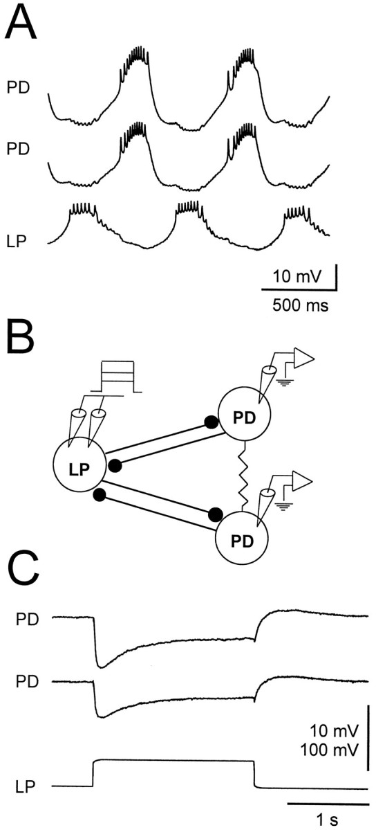
Inhibitory synaptic connections from the LP neuron to the PD neurons. A, In normal saline, the LP and the two PD neurons bursting in alternation. The most hyperpolarized point was −70 mV for the top PD neuron, −65 mV for the bottom PD neuron, and −60 mV for the LP neuron. B, Schematic drawing of the synaptic connections between the LP and PD neurons and the experimental setup. The two PD cells are electrically coupled and form reciprocally inhibitory synaptic connections with the LP neuron. The LP neuron membrane potential was clamped with two electrodes, and the membrane potentials of both PD neurons were monitored in current clamp.C, In TTX, the gIPSP evoked in each PD neuron as the LP neuron membrane potential is stepped from −50 to −10 mV. The gIPSP consists of a transient and a persistent component and is followed by a small rebound depolarization. The two PD neurons had an initial membrane potential of −24 mV. Vertical bar, 10 mV (PDs) and 100 mV (LP).
We studied the effect of the amplitude of the LP neuron depolarization on the amplitude of the early and persistent components of the gIPSP. The presynaptic LP neuron was held at −50 mV, and a sequence of 1.75 sec voltage steps, to voltages ranging from −45 to 0 mV, was applied (Fig. 3A). Changing the holding potential from −50 to −80 mV had a negligible effect on the amplitude of the gIPSP (data not shown).
Fig. 3.
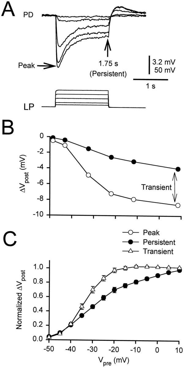
Persistent and transient components of the gIPSP.A, The LP neuron was held at −50 mV, and a sequence of voltage steps, to voltages ranging from −45 to 0 mV, was applied. The amplitude of the gIPSP in the PD cell was measured at the peak and at the end of the pulse (1.75 sec). The initial membrane potential of the PD neuron was −49 mV. Vertical bar, 3.2 mV (PD) and 50 mV (LP).B, The amplitudes at the peak (open circles) and at 1.75 sec (filled circles) of the traces in A are plotted against the presynaptic potential. The amplitude measured at 1.75 sec (the persistent component) was subtracted from the peak amplitude to obtain the transient component (double-headed arrow).C, Both components were normalized to their respective values at +10 mV to obtain the I/O curves (mean ± SEM). The I/O curve of the transient component (open triangles) had a steeper slope and a more hyperpolarized midpoint than that of the persistent component (filled circles).
Figure 3B shows the peak amplitude (open circles) and the amplitude of the gIPSP at 1.75 sec (filled circles) of the traces in Figure3A plotted against the presynaptic potential. The I/O curves for the persistent (filled circles, 1.75 sec) and transient (open triangles, peak minus persistent) components of the gIPSPs of 13 cells are shown in Figure 3C(mean ± SEM). In each experiment, the gIPSPs were normalized with respect to the peak amplitude of the gIPSP in response to a step of the LP neuron to +10 mV. The transient and persistent components of the gIPSP had a sigmoidal dependence on the presynaptic potential. As the presynaptic potential was increased, the amplitude of the persistent component increased more gradually than that of the transient component. We fit the I/O curves for each experiment with sigmoidal functions of the form:
| S1+e−(V−Vmid)k, | Equation 1 |
|---|
where S is the saturation level of the sigmoid,V is the independent variable, _V_midis the half-maximum voltage, and 1/k describes the slope of the sigmoid at V_mid. The values of_V_mid and k for the I/O curves were (in mV, mean ± SEM; n = 15):V_mid = −32.15 ± 0.68 and_k = 5.86 ± 0.31 for the transient component and_V_mid = −26.96 ± 1.45 and_k = 9.25 ± 0.73 for the persistent component. The I/O curves of the transient and persistent components were different (two-way ANOVA, p < 0.01); the transient I/O curve rose at a lower potential and was steeper than the curve of the persistent component.
Depression and recovery of the gIPSP in response to square pulses
We next injected a train of 500 msec, 40 mV voltage pulses (from a baseline of −50 mV) into the LP neuron and varied the duration of the interval between pulses (Fig. 4). With shorter intervals, the synapse showed depression; the amplitude of the gIPSP for the second and subsequent pulses was smaller than that of the first gIPSP. The degree of recovery from depression depended on the interval between the pulses. Figure 4A shows the postsynaptic responses to trains of pulses with intervals of 2 sec (left) and 250 msec (middle) and to a single long pulse (right). Figure 4B shows the depression of the gIPSP amplitude in response to trains of pulses at different intervals plotted against time. This depression is represented as the ratio of each peak amplitude to the amplitude of the first peak. This ratio was independent of the duration of the pulse used and depended only on the intervals between pulses. The decay of the gIPSP in response to a single long pulse (normalized with respect to the peak) is also shown. To quantify the time of recovery from synaptic depression, we compared the amplitudes of the first gIPSP peaks with those of the second gIPSP peaks. Figure 4C shows the ratio of these amplitudes plotted against the interval between the pulses (mean ± SEM; n = 10). A recovery of >90% required intervals of 4 sec or longer. Such intervals exceed the characteristic period of length of 0.5–1 sec when the pyloric rhythm is strongly active.
Fig. 4.

Depression of the gIPSP in response to trains of square pulses. A, Synaptic responses to trains of 500 msec pulses with intervals of 2 sec (left) and 250 msec (middle) and to a single long pulse (right). The PD neuron initial membrane potential was −48 mV. Vertical bar, 6 mV (PD) and 60 mV (LP). B, Depression of the synaptic response represented as the ratio of each peak amplitude to the amplitude of the first peak for different intervals. Also shown is the decay of the response to a single long pulse normalized to the peak (representing interval = 0).C, Recovery from synaptic depression measured as the ratio of second to first peaks versus the interval (n = 10, mean ± SEM).
The I/O curve of the LP to the PD neurons in response to realistic LP waveforms
Unlike spike-mediated synapses, there is no stereotyped waveform to use in studying graded synaptic transmission. Square pulses are the easiest waveforms to generate but are not necessarily the best to characterize the temporal dynamics of graded synapses (Olsen and Calabrese, 1996). During normal oscillations, the membrane potential of pyloric neurons shows smooth envelopes of slow wave depolarizations on which action potentials are superimposed (Fig. 2A). The synaptic response to a natural waveform may be different from the response to a square pulse. This motivated us to use realistic waveforms (see Materials and Methods) to voltage clamp the presynaptic cell.
Figure 5A presents a comparison of the responses to 1.75 sec square pulses and to 1 Hz realistic waveforms at various amplitudes. The average voltage of the realistic waveforms injected was −50 mV, the same as the holding potential for the pulses. The peak potential was used as the presynaptic voltage in the experiments shown in Figure 5, B and C. The amplitude of the gIPSP response to the realistic LP waveform increased gradually to a saturated level with the presynaptic amplitude. Figure5B shows the gIPSP amplitudes in one experiment in response to realistic 1 Hz LP waveforms and to 1.75 sec square pulses plotted against the presynaptic potential. Note that the peak amplitude of the gIPSP in response to the LP waveform is only slightly less than that of the peak gIPSP resulting from a pulse and is considerably larger than the persistent value at the same level of presynaptic depolarization. We normalized the amplitudes (see Fig. 5B) to their respective maximums to obtain the normalized I/O curve for LP waveforms and square pulses (Fig. 5C). The normalized I/O curves for the LP waveforms of each experiment were fit with sigmoidal functions given by Equation 1. The values of V_mid and_k obtained were (in mV, mean ± SEM; _n_= 8): V_mid = −32.18 ± 1.19 and_k = 5.15 ± 0.31. The I/O curve of the LP waveform was different from both the transient and the persistent I/O curves for pulses (two-way ANOVA, p < 0.01).
Fig. 5.
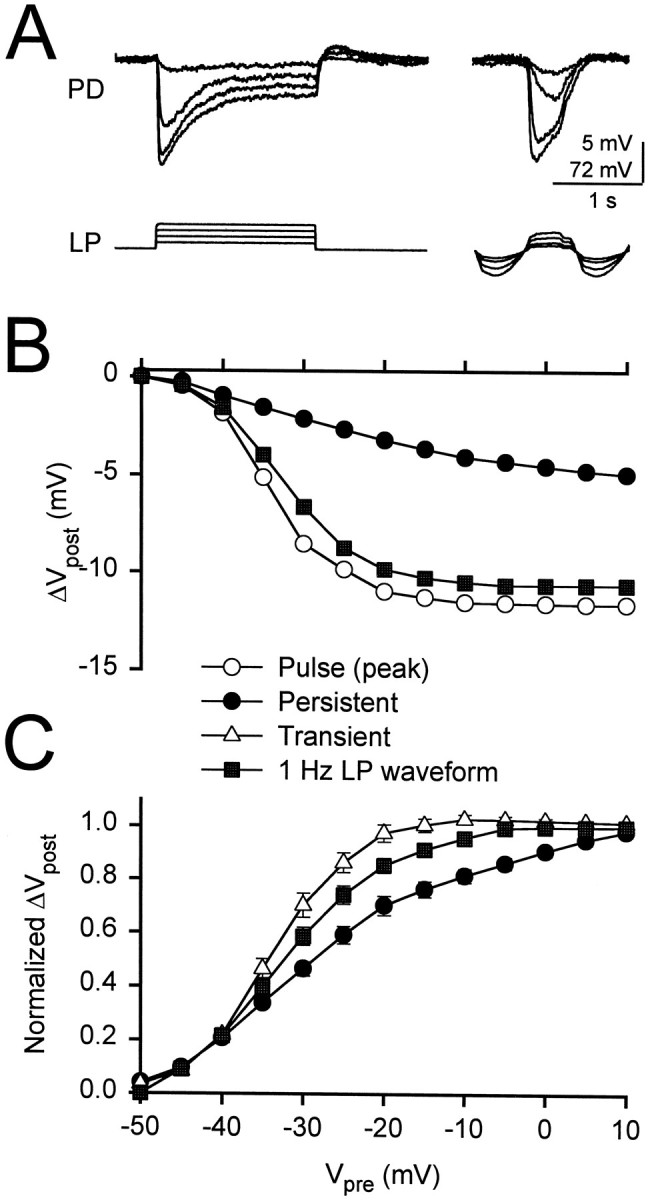
Comparison of I/O curves for square and realistic waveforms. A, A comparison of the responses to 1.75 sec square pulses (left) and to 1 Hz LP waveforms (right). The holding potential of the square pulses and the average of the LP waveforms was −50 mV. The initial membrane potential of the PD neuron was −43 mV. Vertical bar, 5 mV (PD) and 72 mV (LP). B, Amplitudes of the responses to a square pulse [open circles, peak; filled circles, 1.75 sec (the persistent component)] and to an LP waveform (filled squares). C, The normalized I/O curves for the LP waveform and for square pulses (mean ± SEM; n = 8). The normalized I/O curve for the LP waveform (filled squares) falls between those of the persistent (filled circles) and transient (open triangles) components of the square pulse.
For trains of pulses in response to periodic stimulation using the LP waveform, the synapse showed depression over time. The peak amplitude of the gIPSP decayed from its value during the first cycle to a constant steady state value (Fig. 6A). Note that the steady state gIPSP defined here is not the same as the persistent component of the gIPSP measured at the end of a long pulse. In each experiment, we averaged the last four cycles to measure the amplitude of the steady state gIPSP. Figure 6B shows the average amplitudes of the first (filled circles) and the steady state (open circles) gIPSPs in response to a 1 Hz LP waveform plotted against the maximum presynaptic potential (n = 7). We normalized the amplitudes shown in Figure 6B to their respective maximums to obtain the normalized I/O curves (Fig.6C) and fit the I/O curves of each experiment with sigmoidal functions given by Equation 1. The values obtained were (in mV, mean ± SEM; n = 7): _V_mid = −32.18 ± 1.19 and k = 5.15 ± 0.31 for the first peak and V_mid = −31.96 ± 1.15 and_k = 5.89 ± 0.32 for the steady state. The I/O curves for the first and steady state gIPSP were not significantly different.
Fig. 6.
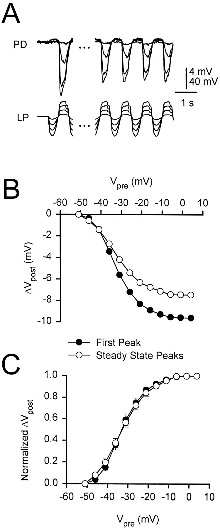
Synaptic depression does not affect the normalized I/O curve. A, Synaptic response to 1 Hz LP waveforms at different amplitudes. The responses to the first cycle (left) and the average of the last four cycles (right, defined as the steady state) of a 20 sec LP waveform are shown. The initial membrane potential of the PD neuron was 0 mV. Vertical bar, 4 mV (PD) and 40 mV (LP). B, Amplitudes of the responses to the first cycle (filled circles) and the steady state (open circles) of the 1 Hz LP waveform. C, The normalized I/O curves (mean ± SEM; n = 7) for the first cycle and the steady state of the LP waveform. The curves are not different (two-way ANOVA, p = 0.996).
The effect of the duty cycle on the amplitude of the gIPSP
The duty cycle of the presynaptic waveform affected the gIPSP amplitude. The duty cycle of an LP waveform was defined as the percentage of the period that the waveform was above/below its mean membrane potential. In the experiments shown in Figure7, the LP neuron was voltage-clamped using two LP waveforms of different duty cycles (55/45 and 35/65). These two duty cycles represent the upper and lower bounds of the LP neuron duty cycles measured in 17 experiments (with inputs from the commissural ganglia remaining attached). The two waveform trajectories spanned the same voltage range (−32 to −72 mV). Figure 7A shows an example of the response to the two duty cycles at 1.5 Hz. Figure7B shows the amplitude of the steady state gIPSP as a function of frequency for the duty cycles of 55/45 (open circles) and 35/65 (filled circles). At all frequencies tested, the amplitude of the gIPSP for the 35/65 duty cycle waveform was larger than that for the 55/45 duty cycle waveform (two-way ANOVA, p < 0.001; _n_= 11).
Fig. 7.
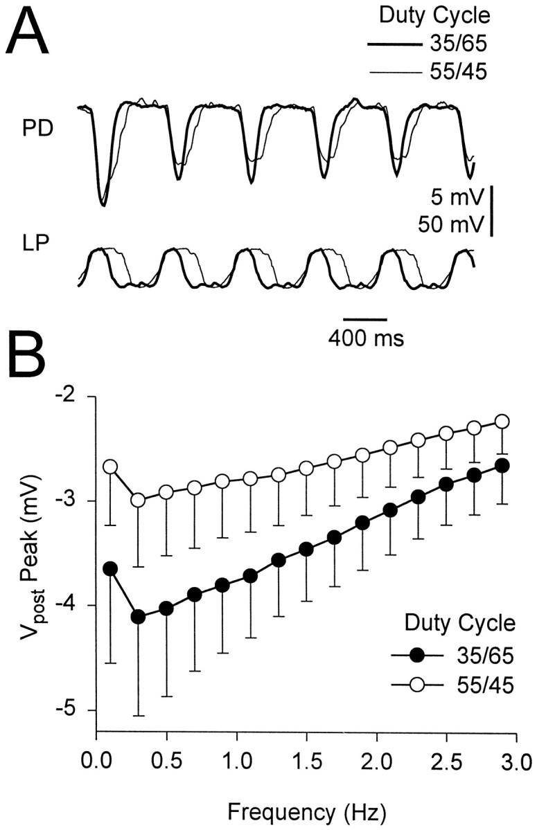
Dependence of the amplitude of the gIPSP on duty cycle. A, Comparison of the synaptic response to 1.5 Hz LP waveforms with duty cycles of 35/65 (thick traces) and 55/45 (thin traces). For both duty cycles, the presynaptic voltage is between −32 and −72 mV. The initial potential of the PD neuron was −21 mV. Vertical bar, 5 mV (PD) and 50 mV (LP).B, Amplitude of the gIPSP for both duty cycles of the LP waveform plotted versus the frequency of the waveform (mean ± SEM; n = 11). At all frequencies the amplitude of the gIPSP in response to the 35/65 waveform was larger than that in response to the 55/45 waveform.
Frequency dependence of synaptic depression
To illustrate directly the effect of frequency on synaptic depression, we now plot a comparison of the response to a first presynaptic depolarization with the response obtained at steady state. Figure 8A shows the dependence of the first (filled circles) and steady state (open circles) gIPSP amplitudes on frequency for square pulses. Amplitudes obtained in each experiment are normalized by the value at the reference amplitude 0.1 Hz (_A_ref). As expected, the response to the first pulse in the train had a constant amplitude, but the response at steady state decayed linearly with frequency (slope = −0.19 ± 0.02 sec, mean ± SEM; n = 5).
Fig. 8.
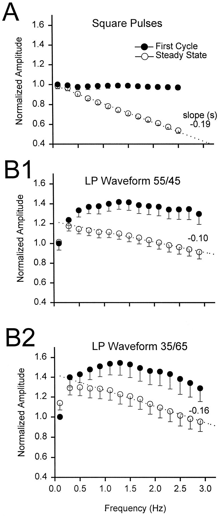
Effect of frequency on the gIPSP amplitude.A, Peak amplitude of the gIPSP in response to trains of square pulses at different frequencies (mean ± SEM;n = 5). Data are normalized with respect to_A_ref, the amplitude of the response at 0.1 Hz. The response to the first pulse (filled circles) was identical at all frequencies. The steady state response (open circles) decayed linearly with increasing frequencies (dashed line, slope = −0.19 sec).B1, B2, Peak amplitude of the gIPSP in response to LP waveforms (duty cycles, 55/45 in B1 and 35/65 in_B2_) plotted against frequency (n = 14 in B1; n = 8 in_B2_, mean ± SEM). Data are normalized with respect to _A_ref. The response to the first injected waveform (filled circles) was limited at frequencies <1 Hz, increased with frequency, and was saturated at ∼1.4 × _A_ref for the duty cycle of 55/45 and at ∼1.45 × _A_ref for the duty cycle of 35/65. The steady state response (open circles, average of the last four responses) was limited at low frequencies but peaked at ∼0.3 Hz and decayed linearly at higher frequencies (dashed lines, slope = −0.10 sec for the duty cycle of 55/45 and −0.16 sec for the duty cycle of 35/65).
With realistic waveforms, the dependence of first and steady state gIPSP amplitudes on frequency was more complex. Figure8B1 shows the dependence of the first and steady state gIPSP amplitudes on frequency for the LP waveform with a duty cycle of 55/45. Amplitudes obtained in each experiment are normalized by _A_ref for this waveform. As frequency was increased, the amplitude of the first gIPSP increased, and at frequencies >0.4 Hz, the amplitude stabilized to a constant level of ∼1.4 × _A_ref (no frequency dependence above 0.4 Hz; Tukey test, p > 0.01; _n_= 14). The initial increase in the amplitude of the first gIPSP is attributable presumably to the slow rise of the presynaptic waveform at very low frequencies, resulting in the inactivation of presynaptic Ca2+ currents that mediate synaptic transmission. In contrast, as frequency was increased, the steady state gIPSP increased to ∼1.2 × _A_ref but decayed linearly at frequencies above 0.3 Hz (slope = −0.10 ± 0.02 sec, mean ± SEM; n = 14). Similar results were obtained for an LP waveform with a duty cycle of 35/65 (Fig.8B2). The first gIPSP amplitude stabilized to a constant level of ∼1.45 × _A_ref (no frequency dependence above 0.2 Hz; Tukey test, p > 0.01; n = 8); the steady state gIPSP increased to ∼1.3 × _A_ref but decayed linearly at frequencies >0.3 Hz (slope = −0.16 ± 0.03 sec, mean ± SEM; n = 8).
The effect of frequency on the phase of the peak gIPSP
The frequency of the injected waveform affected not only the amplitude of the gIPSP but also its shape and, in particular, its rise, decay, and time to peak. We analyzed the gIPSP waveform at frequencies from 0.1 to 3.0 Hz for both 55/45 and 35/65 duty cycles. In Figure9A, we show a sample response to the 35/65 LP waveform at 0.2, 0.8, and 2.4 Hz. To elucidate the difference in the shape of the gIPSP at different frequencies, we rescaled time so that the traces of the LP voltages could be superimposed. We define Δ_t_ as the difference between the peak gIPSP (Fig.9A, upper traces) and the peak of the LP waveform (Fig. 9A, lower trace). At 0.2 Hz, the gIPSP peak was advanced (Δ_t_ < 0) with respect to the peak of the LP waveform; at 2.4 Hz, it was delayed (Δ_t_ > 0); at 0.8 Hz, it was approximately aligned (Δ_t_ = 0). This dependence of phase (Δ_t_/period) on frequency was affected by the duty cycle of the LP waveform, as shown in Figure 9B. The phase is plotted for frequencies ranging from 0.1 to 3 Hz for both 35/65 (filled circles) and 55/45 (open circles) LP waveforms. At frequencies <1.5 Hz, the postsynaptic response was more phase-advanced (negative phase) with respect to the LP waveform with the 55/45 duty cycle compared with the 35/65 duty cycle (two-way ANOVA, p < 0.01;n = 10). The zero-phase frequency (the frequency for which Δ_t_ = 0, calculated by linear interpolation between the two frequencies immediately above and below the zero phase) was 1.39 ± 0.17 Hz (mean ± SEM) for the 55/45 duty cycle waveform, a value significantly larger than 0.92 ± 0.09 Hz (mean ± SEM), the value for the 35/65 duty cycle waveform (p < 0.002, paired t test;n = 10). In calculating phase, we chose the peak of the LP waveform as a point of reference. Choosing any other point at a fixed phase of the LP waveform would just shift the phase (Δ_t_/period) traces in Figure 9B by fixed constant values.
Fig. 9.
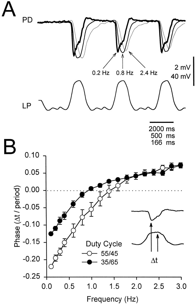
The effect of frequency on the phase of the steady state gIPSP. The phase of the gIPSP is defined as the time lag (Δ_t_) between the gIPSP peak and the peak of the LP waveform (B, inset), normalized by the period of the waveform. A, gIPSP (recorded at −49 mV) in response to a periodic LP waveform with the 35/65 duty cycle at 0.2 Hz (thick trace), 0.8 Hz (medium trace), and 2.4 Hz (thin trace). The time axis is scaled in each case so that the three LP waveforms are superimposed. The gIPSP peaked_before_ the peak of the 0.2 Hz LP waveform (Δ_t_ < 0) but after_ the peak of the 2.4 Hz waveform (Δ_t_ > 0). At 0.8 Hz, the two peaks were approximately aligned (Δ_t = 0). Vertical bar, 2 mV (PD) and 40 mV (LP). B, Plot of phase versus frequency for waveforms of the duty cycles of 35/65 (filled circles) and 55/45 (open circles) (mean ± SEM; n = 10).
The effect of duty cycle and frequency on the shape of the gIPSP
Until this point we have focused on the amplitude of the gIPSP, because this is the usual parameter used to express synaptic strength. However, the duration of the synaptic potential may be critical for determining when the PD neurons can resume firing after LP neuron inhibition. Therefore, it is important to study the effect of frequency on the duration of the gIPSP as well. Given the complex waveforms of the postsynaptic responses, it is not trivial to decide exactly how to measure the duration of the gIPSP or, for that matter, how to express a “synaptic weight over time” that best captures the time and amplitude information together. The simplest strategy is to calculate the integral. In Figure 10, we show the ratio of these integrals for the duty cycles of 55/45 and 35/65. The ratio of the postsynaptic integrals (filled squares) was 20–30% smaller than the ratio of the presynaptic integrals (open triangles) and was fairly independent of frequency. This reduction implies that the synapse acts as a buffer to reduce the difference of integrals from the input to the output at all frequencies.
Fig. 10.
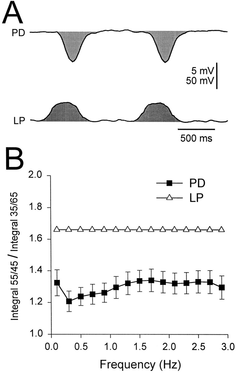
The ratio of integrals for different duty cycles.A, An example of the integrals calculated for the presynaptic LP waveforms and the gIPSP in PD neurons (shaded areas). Vertical bar, 5 mV (PD) and 50 mV (LP).B, The ratios of integrals for duty cycles of 55/45 and 35/65 for the LP waveforms (open triangles) and the PD responses (filled squares) are shown.
The integral alone, however, does not distinguish between amplitude and duration of the synaptic potential. Therefore, we have defined “equivalent rectangles” that attempt to capture the time and amplitude dependence of the integrals. The equivalent rectangle of a waveform (Fig. 11A) is defined as a rectangle of length _t_equiv (a measure of the waveform duration) and height _V_avg (a measure of the average amplitude of the waveform). To calculate_t_equiv, we first calculate the integral of the waveform in each cycle and find the time of the half-integral. This time is then doubled to give _t_equiv._V_avg is calculated in each cycle by dividing the integral of the waveform by _t_equiv. Therefore the area represented by the product of _t_equivand _V_avg is equal to the integral, but this area is now expressed such that it weights appropriately the average amplitude and duration of the waveform.
Fig. 11.

Representation of LP waveforms and PD gIPSPs with equivalent rectangles. The equivalent rectangle of a waveform is defined as a rectangle of length _t_equiv(a measure of the waveform length) and height_V_avg (a measure of the average amplitude of the waveform), in which _t_equiv is twice the time that divides the waveform in two parts with equal integrals, and_V_avg is the ratio of the integral of the waveform in one period to _t_equiv. The area of the equivalent rectangle is therefore equal to the integral of the waveform during one cycle. A, Equivalent rectangles superimposed on one cycle of a 0.2 Hz LP waveform (bottom) and the PD response (top). The integral of the LP waveform is measured from its minimum, and the integral of the PD response is measured from its baseline (−23 mV). Vertical bar, 2 mV (PD) and 20 mV (LP). B, Equivalent rectangles for LP waveforms (bottom) and PD responses (top, mean ± SEM; n = 14) at frequencies of 0.2, 0.8, 2.0, and 2.8 Hz. In each case, two duty cycles are superimposed: 55/45 (light gray) and 35/65 (dark gray). The height of the equivalent rectangles for PD responses are _V_avg values normalized to the _V_avg of the response to the 0.1 Hz LP waveform with the duty cycle of 55/45 (_A_ref). Vertical bar,_A_ref (PD) and 40 mV (LP). C,_V_avg normalized by_A_ref (mean ± SEM;n = 14) plotted against frequency for gIPSPs in response to LP waveforms with duty cycles of 55/45 (open circles) and 35/65 (filled circles).D, _t_equiv normalized by period (mean ± SEM; n = 13) plotted against frequency for gIPSPs in response to LP waveforms with duty cycles of 55/45 (open circles) and 35/65 (filled circles). Dotted lines show the normalized_t_equiv values for the LP waveforms (0.41 for the 35/65 duty cycle and 0.61 for the 55/45 duty cycle).
Figure 11B shows the equivalent rectangles of the presynaptic waveform (bottom) and the postsynaptic response (top) at frequencies of 0.2, 0.8, 2.0, and 2.8 Hz (mean ± SEM; n = 14) for waveforms with the duty cycles of 35/65 (dark gray) and 55/45 (light gray). To remove variability among experiments, we normalized _V_avg values of postsynaptic equivalent rectangles to the _V_avg of the 0.1 Hz waveform with the duty cycle of 55/45 (the_A_ref). At all four frequencies, the_V_avg values obtained for LP waveforms with the duty cycle of 35/65 were larger than the corresponding values obtained for the waveforms with the duty cycle of 55/45. As frequency increased, the _V_avg of response to both the 55/45 and the 35/65 duty cycle waveforms increased to a peak at 0.8 Hz and then decreased. As the frequency increased, _t_equiv of both the presynaptic waveform and the postsynaptic response decreased. This decrease was more moderate for the postsynaptic responses. The dotted vertical lines indicate the _t_equiv values of the presynaptic waveforms and the postsynaptic responses.
These results are maintained across the whole range of frequencies tested. In Figure 11C, _V_avg is plotted as a function of frequency for the two duty cycles. At all frequencies, _V_avg of the 35/65 (filled circles) duty cycle was larger than_V_avg of the 55/45 (open circles) duty cycle (two-way ANOVA, p < 0.05; n = 14). For both duty cycles,_V_avg reached a maximum at 0.8 Hz. Figure11D shows the plot of the ratio of_t_equiv to period (defined here as the “normalized _t_equiv”) as a function of frequency. At all frequencies, the _t_equivgenerated by the 55/45 (open circles) duty cycle LP waveform was larger than that produced by the 35/65 (filled circles) duty cycle LP waveform (two-way ANOVA, p < 0.01). The horizontal dotted lines show the normalized _t_equiv for the presynaptic waveforms. As frequency increased, the normalized_t_equiv of the postsynaptic gIPSP approached the normalized _t_equiv of the presynaptic waveform. For the 35/65 duty cycle waveform, the postsynaptic normalized_t_equiv crossed that of the presynaptic waveform at ∼1.7 Hz.
The effect of spike-mediated IPSPs
Because we were interested in graded transmission, the waveforms that we used to mimic realistic oscillations in the cells were averaged and low-pass filtered so that the action potentials were eliminated. To study the additional effect of presynaptic action potentials on the IPSP, we compared the response to filtered waveforms injected in the LP cell with the response to nonfiltered waveforms. In Figure12A, we show the response to superimposed nonfiltered and filtered waveforms. Compared with the response to the filtered waveform, the response to the nonfiltered waveform was jagged (corresponding one to one to the injected spikes), was ∼35% larger, and was faster to rise (maximum slope of rise was ∼100% larger).
Fig. 12.

Effect of simulated spike-mediated IPSPs. A, IPSPs in response to 1 Hz LP waveforms with the spikes filtered out (smooth trace) and with the spikes not filtered (jagged trace). The nonfiltered waveform elicited an IPSP that was larger in amplitude than that of the filtered waveform and was jagged. The jaggedness corresponded one-to-one to IPSPs elicited by the simulated spikes. The jagged trace was also faster to rise. Vertical bar, 10 mV (PD) and 50 mV (LP). B, The gIPSPs in response to the filtered LP waveforms from A compared with the response to the same waveform (bottom LP trace), amplified to the average of the nonfiltered waveform in A (middle LP trace), and amplified to the outer envelope(maximum) of the nonfiltered waveform in A (top LP trace). The larger waveforms elicited gIPSPs that were larger in amplitude and faster to rise. The large amplitude and fast rise of the response to the nonfiltered waveform in_A_ was accounted for by the response to the average of that waveform (middle LP trace). The membrane potential of the PD neuron was −42 mV.
Was the larger amplitude in the response to the nonfiltered waveform merely caused by the larger average potential of the input waveform, or was this response caused by other factors such as the slope of the LP waveform or the existence of spikes? To answer this question, we injected the LP neuron with filtered waveforms that had the same_maximum_ or the same average amplitude as the nonfiltered waveform, and we compared the result with the injection with the original “envelope” filtered waveform (Fig.12B). The increase in the amplitude of the IPSP was fully compensated for by the larger average input waveform (Fig.12B, middle LP trace). Surprisingly, the filtered waveform with the same average amplitude as the nonfiltered one also produced a sharp initial rise in the IPSP, similar to the response to the nonfiltered waveform. The envelopes of the synaptic response to the nonfiltered waveform with spikes (Fig.12A, jagged PD trace) and to the filtered waveform without spikes but with the same average amplitude (Fig. 12B, middle PD trace) were approximately equal, both in amplitude and in rise time. The filtered waveform with the same maximum (Fig.12B, top LP trace) produced a disproportionately larger IPSP than the nonfiltered waveform.
DISCUSSION
Graded synaptic transmission is a common feature of many invertebrate sensory and motor networks (Pearson and Fourtner, 1975;Burrows and Siegler, 1978; DiCaprio, 1989; Nadim et al., 1995; Olsen et al., 1995) and of the vertebrate retina (Roberts and Bush, 1981). Synaptic potentials in the stomatogastric nervous system, like those in the leech (Nadim et al., 1995; Olsen et al., 1995), are both graded and spike-mediated. Previous work on graded transmission in the STG suggested that most of the transmitter release was graded with a relatively minor spike-mediated component (Graubard et al., 1980, 1983,1989). Our research provides an excellent opportunity to develop the frameworks needed for a detailed description of the dynamic properties of graded synaptic transmission.
Like spike-mediated synapses, graded synapses exhibit use-dependent changes in efficacy. However, the study of graded synaptic transmission introduces a number of challenging issues that are not confronted in the study of spike-mediated synapses. Transmission at spike-mediated synapses depends primarily on the timing of action potentials arriving at the presynaptic terminal and secondarily on changes in action potential duration and waveform, when they occur. At a graded synapse, both the timing and the waveform of the presynaptic depolarization are always important. Here we extend the discussion and analysis of short-term synaptic plasticity to the richer domain of graded synaptic transmission.
We began by investigating the postsynaptic response to square pulses of presynaptic depolarization. For trains of brief pulses, these synapses showed depression similar to the depression that can be seen at some spike-mediated synapses (Del Castillo and Katz, 1954; Betz, 1970;Charlton et al., 1982; Magleby, 1987; Thomson and Deuchars, 1994;Abbott et al., 1997). However, as the duration of each pulse was extended, depression was seen not only from one pulse to another but within a single extended pulse. As a result, the response to a single extended pulse consists of transient (depressing) and sustained (nondepressing) components. Ninety percent recovery from depression takes ∼4 sec, which means that when the pyloric period is <4–5 sec (most of the time), the synapse is continuously depressed to some degree. The fact that the synapse is neither full strength nor maximally depressed within the natural frequency range (0.1–2.5 Hz) enables it to be strengthened or weakened by variations in frequency, suggesting a functional role.
Almost all of the previously published work studying graded synaptic transmission in the stomatogastric nervous system used single, long, square presynaptic current pulses (Maynard and Walton, 1975; Graubard, 1978; Graubard et al., 1980, 1983; Johnson and Harris-Warrick, 1990;Johnson et al., 1991, 1995). Our study reveals that the amplitude of the postsynaptic response depends on the specific shape of the presynaptic waveform. In particular, the peak amplitude is sensitive to the slope of the rising phase of the presynaptic depolarization. This sensitivity means that square pulses, with their extremely high initial slopes, are inappropriate waveforms. Correlation of presynaptic Ca2+ currents with graded postsynaptic currents in leech heart interneurons (Angstadt and Calabrese, 1991) and subsequent modeling of that network (Nadim et al., 1995) indicated that graded synapses are sensitive to the slope of the presynaptic waveform. This sensitivity was experimentally demonstrated (Olsen and Calabrese, 1996). One message of our work is that it is important to use presynaptic waveforms typical of natural conditions when studying graded synapses. We used prerecorded presynaptic waveforms from rhythmically active preparations that we scaled to generate different amplitudes and frequencies. Our work, summarized below, was based on these “natural” waveforms.
Effect of duty cycle and waveform
A somewhat surprising result was that increasing the duty cycle of the presynaptic neuron decreases the peak amplitude of the evoked gIPSP (Fig. 7). This is presumably because of the increased recovery time between pulses and the more steeply rising slope of the waveform with the shorter duty cycle. The dependence of postsynaptic response on the initial slope of the presynaptic waveform may arise because the Ca2+ currents that are responsible for release of transmitter inactivate during slowly rising depolarizations. The use of the equivalent rectangle representation (Fig. 11B) allowed us to decompose the postsynaptic response into an average voltage, _V_avg, and an equivalent duration, _t_equiv. As expected, when the duty cycle increases, the postsynaptic _t_equiv also increases, but again, nonintuitively, the postsynaptic_V_avg decreases. It is possible that alterations in the intrinsic properties of the postsynaptic neuron (by modulatory substances or by network dynamics) may influence whether the time course (_t_equiv) or amplitude (_V_avg) of the synaptic potential is more important. Specifically, the trajectory of the recovery from the gIPSP will interact with currents such as _I_h,_I_A, and low-threshold Ca2+ currents that influence when the postsynaptic cell fires after inhibition.
Effect of frequency
We found that the frequency of the presynaptic waveform affects the amplitude (peak and _V_avg) of the postsynaptic response in an interesting way. As frequency increases, the amplitude of the gIPSP first increases and then decreases. The initial increase may be caused by less inactivation of presynaptic Ca2+ currents during the rise of the LP waveform at higher frequencies. The shorter recovery period, as frequency increases further, is probably responsible for the subsequent decrease in the gIPSP amplitude. We also found that frequency influences the gIPSP time course (time to peak and _t_equiv). As the frequency increases, the waveforms of the presynaptic and postsynaptic responses become better aligned (Fig. 11). This means that the time course of the postsynaptic response tracks that of the presynaptic depolarization best at high frequencies (Fig.11B).
The role of the LP neuron in controlling pyloric frequency
It is natural to ask what effect the synaptic dynamics investigated here has on the operation of the pyloric network of the STG. Although we do not have a definitive answer to this question, a number of features are suggestive. The LP to PD synapse provides the only feedback to the AB and PD pacemaker from other pyloric neurons, so it is well placed to affect the frequency and phase relationships of the three-component rhythm. Under some modulatory conditions, increasing the duty cycle of the LP neuron slows down the pyloric frequency (Weimann et al., 1997), but this is not always the case (Hooper and Marder, 1987). Phase response curves obtained by firing single LP neuron action potentials (Ayers and Selverston, 1979) show a phase advance when the LP neuron fires during or just after the PD neuron burst but shows a phase delay when the LP neuron fires late in the cycle. However, because graded synaptic transmission arising from the slow wave potential of the LP neurons is probably the dominant source of synaptic transmission, it is essential to understand the dynamics of graded transmission and its role in frequency and phase regulation before we can fully appreciate the role of LP neuron to PD neuron feedback in the pyloric network.
The kinetics of depression and its recovery at the synapse studied here are tuned so that synaptic transmission is sensitive to frequency and to duty cycle in the range over which the pyloric network normally operates. When the pyloric rhythm is slow, the LP neuron is either silent or fires only one or two spikes or bursts. Under these conditions, the LP to PD synapse will be relatively constant. As the pyloric frequency increases or when the LP duty cycle increases, the amount of depression also increases. In our paradigms, synaptic depression is almost totally attained within one or two cycles, depending on frequency. This implies that the amplitude of the synapse will follow quickly any rapid changes in frequency produced by synaptic or neuromodulatory inputs. The complex effects of frequency and duty cycle on the gIPSP peak, integral,_t_equiv, and _V_avgmake it difficult to predict how different LP waveforms will affect the pyloric period and phasing without more detailed modeling studies. However, the results reported here suggest that the synaptic dynamics we have measured should, in general, have a buffering effect on fluctuations of rhythm and phase within the network.
Previous work has shown that modulatory substances can alter the peak amplitude of the gIPSP evoked by square pulses in the STG (Johnson and Harris-Warrick, 1990; Johnson et al., 1991, 1995). Because, in principle, a modulatory substance could alter the kinetics of depression, it will be interesting to determine how modulatory substances alter graded transmission studied with natural waveforms of different frequencies.
It is a truism that network dynamics depend on the interaction of synaptic and intrinsic membrane properties (Marder and Calabrese, 1996). Many attempts have been made to measure synaptic strength between pattern-generating neurons, with the presumption that these measurements would be useful in constructing models of circuit behavior (Getting, 1989). Unfortunately, measurements of synaptic strength are most easily made in inactive networks and then extrapolated to networks with ongoing activity. Models of networks using spike-mediated and/or graded transmission must be built with synaptic models that incorporate the appropriate time-dependent alterations in synaptic function, or they are unlikely to be adequate for explaining the dynamics of networks.
Footnotes
This research was supported by National Institute of Neurological Diseases and Stroke Grant NS17813 and National Institute of Mental Health Grant MH46742, the Sloan Center for Theoretical Neurobiology, and the W. M. Keck Foundation. The first two authors contributed equally to this work. We thank Dr. Jorge Golowasch for helpful discussions.
Correspondence should be addressed to Dr. Eve Marder, Volen Center, Brandeis University, 415 South Street, Waltham, MA 02254.
REFERENCES
- 1.Abbott LF, Sen K, Varela J, Nelson SB. Synaptic depression and cortical gain control. Science. 1997;275:220–224. doi: 10.1126/science.275.5297.221. [DOI] [PubMed] [Google Scholar]
- 2.Anderson WW, Barker DL. Synaptic mechanisms that generate network oscillations in the absence of discrete postsynaptic potentials. J Exp Zool. 1981;216:187–191. doi: 10.1002/jez.1402160121. [DOI] [PubMed] [Google Scholar]
- 3.Angstadt JD, Calabrese RL. Calcium currents and graded synaptic transmission between heart interneurons of the leech. J Neurosci. 1991;11:746–759. doi: 10.1523/JNEUROSCI.11-03-00746.1991. [DOI] [PMC free article] [PubMed] [Google Scholar]
- 4.Ayers JL, Selverston AI. Monosynaptic entrainment of an endogenous pacemaker network: a cellular mechanism for von Holt’s magnet effect. J Comp Physiol [A] 1979;129:5–17. [Google Scholar]
- 5.Betz WJ. Depression of transmitter release at the neuromuscular junction of the frog. J Physiol (Lond) 1970;206:629–644. doi: 10.1113/jphysiol.1970.sp009034. [DOI] [PMC free article] [PubMed] [Google Scholar]
- 6.Burrows M, Siegler MV. Graded synaptic transmission between local interneurons and motor neurons in the metathoracic ganglion of the locust. J Physiol (Lond) 1978;285:231–255. doi: 10.1113/jphysiol.1978.sp012569. [DOI] [PMC free article] [PubMed] [Google Scholar]
- 7.Charlton MP, Smith SJ, Zucker RS. Role of presynaptic calcium ions and channels in synaptic facilitation and depression at the squid giant synapse. J Physiol (Lond) 1982;323:173–193. doi: 10.1113/jphysiol.1982.sp014067. [DOI] [PMC free article] [PubMed] [Google Scholar]
- 8.Del Castillo J, Katz B. Statistical factors involved in neuromuscular facilitation and depression. J Physiol (Lond) 1954;124:574–585. doi: 10.1113/jphysiol.1954.sp005130. [DOI] [PMC free article] [PubMed] [Google Scholar]
- 9.DiCaprio RA. Nonspiking interneurons in the ventilatory central pattern generator of the shore crab, Carcinus maenas. J Comp Neurol. 1989;185:83–106. doi: 10.1002/cne.902850108. [DOI] [PubMed] [Google Scholar]
- 10.Eisen JS, Marder E. Mechanisms underlying pattern generation in lobster stomatogastric ganglion as determined by selective inactivation of identified neurons. III. Synaptic connections of electrically coupled pyloric neurons. J Neurophysiol. 1982;48:1392–1415. doi: 10.1152/jn.1982.48.6.1392. [DOI] [PubMed] [Google Scholar]
- 11.Eisen JS, Marder E. A mechanism for production of phase shifts in a pattern generator. J Neurophysiol. 1984;51:1375–1393. doi: 10.1152/jn.1984.51.6.1375. [DOI] [PubMed] [Google Scholar]
- 12.Getting PA. Reconstruction of small neural networks. In: Koch C, Segev I, editors. Methods in neuronal modeling. Massachusetts Institute of Technology; Cambridge, MA: 1989. pp. 171–194. [Google Scholar]
- 13.Graubard K. Synaptic transmission without action potentials: input–output properties of a non-spiking presynaptic neuron. J Neurophysiol. 1978;41:1014–1025. doi: 10.1152/jn.1978.41.4.1014. [DOI] [PubMed] [Google Scholar]
- 14.Graubard K, Raper JA, Hartline DK. Graded synaptic transmission between spiking neurons. Proc Natl Acad Sci USA. 1980;77:3733–3735. doi: 10.1073/pnas.77.6.3733. [DOI] [PMC free article] [PubMed] [Google Scholar]
- 15.Graubard K, Raper JA, Hartline DK. Graded synaptic transmission between identified spiking neurons. J Neurophysiol. 1983;50:508–521. doi: 10.1152/jn.1983.50.2.508. [DOI] [PubMed] [Google Scholar]
- 16.Graubard K, Raper JA, Hartline DK. Quantitative analysis of non-spiking synaptic transmission between spiking stomatogastric neurons. Soc Neurosci Abst. 1989;15:1047. [Google Scholar]
- 17.Harris-Warrick RM, Marder E, Selverston AI, Moulins M. Dynamic biological networks. Massachusetts Institute of Technology; The stomatogastric nervous system. Cambridge, MA: 1992. [Google Scholar]
- 18.Hartline DK, Graubard K. Cellular and synaptic properties in the crustacean stomatogastric nervous system. In: Harris-Warrick RM, Marder E, Selverston AI, Moulins M, editors. Dynamic biological networks. The stomatogastric nervous system. Massachusetts Institute of Technology; Cambridge, MA: 1992. pp. 31–85. [Google Scholar]
- 19.Hartline DK, Russell DF, Raper JA, Graubard K. Special cellular and synaptic mechanisms in motor pattern generation. Comp Biochem Physiol. 1988;91C:115–131. doi: 10.1016/0742-8413(88)90177-6. [DOI] [PubMed] [Google Scholar]
- 20.Hooper SL (1997a) Phase maintenance in the pyloric pattern of the lobster (Panulirus interruptus) stomatogastric ganglion. J Comput Neurosci, in press. [DOI] [PubMed]
- 21.Hooper SL (1997b) The pyloric pattern of the lobster (Panulirus interruptus) stomatogastric ganglion comprises two phase maintaining subsets. J Comput Neurosci, in press. [DOI] [PubMed]
- 22.Hooper SL, Marder E. Modulation of the lobster pyloric rhythm by the peptide proctolin. J Neurosci. 1987;7:2097–2112. doi: 10.1523/JNEUROSCI.07-07-02097.1987. [DOI] [PMC free article] [PubMed] [Google Scholar]
- 23.Johnson BR, Harris-Warrick RM. Aminergic modulation of graded synaptic transmission in the lobster stomatogastric ganglion. J Neurosci. 1990;10:2066–2076. doi: 10.1523/JNEUROSCI.10-07-02066.1990. [DOI] [PMC free article] [PubMed] [Google Scholar]
- 24.Johnson BR, Peck JH, Harris-Warrick RM. Temperature sensitivity of graded synaptic transmission in the lobster stomatogastric ganglion. J Exp Biol. 1991;156:267–285. doi: 10.1242/jeb.156.1.267. [DOI] [PubMed] [Google Scholar]
- 25.Johnson BR, Peck JH, Harris-Warrick RM. Distributed amine modulation of graded chemical transmission in the pyloric network of the lobster stomatogastric ganglion. J Neurophysiol. 1995;174:437–452. doi: 10.1152/jn.1995.74.1.437. [DOI] [PubMed] [Google Scholar]
- 26.Magleby K. Short-term changes in synaptic efficacy. In: Edelman GM, Gall WE, Cowan WM, editors. Synaptic function. Wiley; New York: 1987. pp. 21–56. [Google Scholar]
- 27.Marder E, Calabrese RL. Principles of rhythmic motor pattern generation. Physiol Rev. 1996;76:687–717. doi: 10.1152/physrev.1996.76.3.687. [DOI] [PubMed] [Google Scholar]
- 28.Maynard DM. Simpler networks. Ann NY Acad Sci. 1972;193:59–72. doi: 10.1111/j.1749-6632.1972.tb27823.x. [DOI] [PubMed] [Google Scholar]
- 29.Maynard DM, Walton KD. Effects of maintained depolarization of presynaptic neurons on inhibitory transmission in lobster neuropil. J Comp Physiol [A] 1975;97:215–243. [Google Scholar]
- 30.Miller JP, Selverston AI. Mechanisms underlying pattern generation in lobster stomatogastric ganglion as determined by selective inactivation of identified neurons. II. Oscillatory properties of pyloric neurons. J Neurophysiol. 1982a;48:1378–1391. doi: 10.1152/jn.1982.48.6.1378. [DOI] [PubMed] [Google Scholar]
- 31.Miller JP, Selverston AI. Mechanisms underlying pattern generation in lobster stomatogastric ganglion as determined by selective inactivation of identified neurons. IV. Network properties of pyloric system. J Neurophysiol. 1982b;48:1416–1432. doi: 10.1152/jn.1982.48.6.1416. [DOI] [PubMed] [Google Scholar]
- 32.Mulloney B, Selverston AI. Organization of the stomatogastric ganglion in the spiny lobster. I. Neurons driving the lateral teeth. J Comp Physiol [A] 1974a;91:1–32. [Google Scholar]
- 33.Mulloney B, Selverston AI. Organization of the stomatogastric ganglion in the spiny lobster. III. Coordination of the two subsets of the gastric system. J Comp Physiol [A] 1974b;91:53–78. [Google Scholar]
- 34.Nadim F, Olsen ØH, Calabrese RL. Modeling the leech heartbeat elemental oscillator. I. Interactions of intrinsic and synaptic currents. J Comput Neurosci. 1995;2:215–235. doi: 10.1007/BF00961435. [DOI] [PubMed] [Google Scholar]
- 35.Olsen ØH, Calabrese RL. Activation of intrinsic and synaptic currents in leech heart interneurons by realistic waveforms. J Neurosci. 1996;16:4958–4970. doi: 10.1523/JNEUROSCI.16-16-04958.1996. [DOI] [PMC free article] [PubMed] [Google Scholar]
- 36.Olsen ØH, Nadim F, Calabrese RL. Modeling the leech heartbeat elemental oscillator. II. Exploring the parameter space. J Comput Neurosci. 1995;2:237–257. doi: 10.1007/BF00961436. [DOI] [PubMed] [Google Scholar]
- 37.Pearson KG, Fourtner CR. Non-spiking interneurons in walking system of the cockroach. J Neurophysiol. 1975;38:33–52. doi: 10.1152/jn.1975.38.1.33. [DOI] [PubMed] [Google Scholar]
- 38.Raper JA. Nonimpulse-mediated synaptic transmission during the generation of a cyclic motor program. Science. 1979;205:304–306. doi: 10.1126/science.221982. [DOI] [PubMed] [Google Scholar]
- 39.Rezer E, Moulins M. Expression of the crustacean pyloric pattern generator in the intact animal. J Comp Physiol [A] 1983;153:17–28. [Google Scholar]
- 40.Roberts A, Bush BMH. Neurones without impulses. Cambridge UP; Cambridge, UK: 1981. [Google Scholar]
- 41.Selverston AI, Miller JP. Mechanisms underlying pattern generation in the lobster stomatogastric ganglion as determined by selective inactivation of identified neurons. I. Pyloric neurons. J Neurophysiol. 1980;44:1102–1121. doi: 10.1152/jn.1980.44.6.1102. [DOI] [PubMed] [Google Scholar]
- 42.Selverston AI, Russell DF, Miller JP, King DG. The stomatogastric nervous system: structure and function of a small neural network. Prog Neurobiol. 1976;7:215–290. doi: 10.1016/0301-0082(76)90008-3. [DOI] [PubMed] [Google Scholar]
- 43.Thomson AM, Deuchars J. Temporal and spatial properties of local circuits in neocortex. Trends Neurosci. 1994;17:119–126. doi: 10.1016/0166-2236(94)90121-x. [DOI] [PubMed] [Google Scholar]
- 44.Turrigiano GG, Heinzel HG. Behavioral correlates of stomatogastric network function. In: Harris-Warrick RM, Marder E, Selverston AI, Moulins M, editors. Dynamic biological networks. The stomatogastric nervous system. Massachusetts Institute of Technology; Cambridge, MA: 1992. pp. 197–220. [Google Scholar]
- 45.Weimann JM, Skiebe P, Heinzel H-G, Soto C, Kopell N, Jorge-Rivera JC, Marder E. Modulation of oscillator interactions in the crab stomatogastric ganglion by crustacean cardioactive peptide. J Neurosci. 1997;17:1748–1760. doi: 10.1523/JNEUROSCI.17-05-01748.1997. [DOI] [PMC free article] [PubMed] [Google Scholar]