Unsupervised Discovery of Demixed, Low-Dimensional Neural Dynamics across Multiple Timescales through Tensor Component Analysis (original) (raw)
. Author manuscript; available in PMC: 2019 Dec 12.
SUMMARY
Perceptions, thoughts, and actions unfold over millisecond timescales, while learned behaviors can require many days to mature. While recent experimental advances enable large-scale and long-term neural recordings with high temporal fidelity, it remains a formidable challenge to extract unbiased and interpretable descriptions of how rapid single-trial circuit dynamics change slowly over many trials to mediate learning. We demonstrate a simple tensor component analysis (TCA) can meet this challenge by extracting three interconnected, low-dimensional descriptions of neural data: neuron factors, reflecting cell assemblies; temporal factors, reflecting rapid circuit dynamics mediating perceptions, thoughts, and actions within each trial; and trial factors, describing both long-term learning and trial-to-trial changes in cognitive state. We demonstrate the broad applicability of TCA by revealing insights into diverse datasets derived from artificial neural networks, large-scale calcium imaging of rodent prefrontal cortex during maze navigation, and multi-electrode recordings of macaque motor cortex during brain machine interface learning.
Graphical Abstract
In Brief
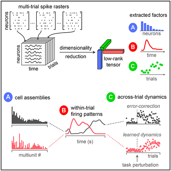
Williams et al. describe an unsupervised method to uncover simple structure in large-scale recordings by extracting distinct cell assemblies with rapid withintrial dynamics, reflecting interpretable aspects of perceptions, actions, and thoughts, and slower across-trial dynamics reflecting learning and internal state changes.
INTRODUCTION
Neural circuits operate over a wide range of dynamical time-scales. Circuit dynamics mediating sensory perception, deci sion-making, and motor control unfold over hundreds of milliseconds (Uchida et al., 2006; Churchland et al., 2012), while slower processes like learning and changes in motivational state can vary slowly over days or weeks (Kleim et al., 1998; Ganguly and Carmena, 2009; Peters et al., 2014). Recent experimental advances enable us to monitor all aspects of this complexity by recording large numbers of neurons at high temporal precision (Marblestone et al., 2013; Kim et al., 2016; Lin and Schnitzer, 2016; Pachitariu et al., 2016; Jun et al., 2017) over long durations (Lütcke et al., 2013; Dhawale et al., 2017), thereby documenting the dynamics of thousands of neurons over thousands of behavioral trials. These modern large-scale datasets present a major analysis challenge: how can we extract simple and interpretable low-dimensional descriptions of circuit dynamics underlying both rapid sensory, motor, and cognitive acts, and slower processes like learning or changes in cognitive state? Moreover, how can we extract these descriptions in an unsupervised manner, to enable the discovery of novel and unexpected circuit dynamics that can vary on a trial-by-trial basis?
Commonly used dimensionality reduction methods focus on reducing the complexity of fast, within-trial firing rate dynamics instead of extracting slow, across-trial structure. A common approach is to average neural activity across trials (Churchland et al., 2012; Gao and Ganguli, 2015), thereby precluding the possibility of understanding of how cognition and behavior change on a trial-by-trial basis. More recent methods, including Gaussian process factor analysis (GPFA) (Yu et al., 2009) and latent dynamical system models (Gao et al., 2016; Pandarinath et al., 2017), identify low-dimensional firing rate trajectories within each trial, but do not reduce the dimensionality across trials by extracting analogous low-dimensional trajectories over trials. Other works have focused on trial-to-trial variability in neural responses (Averbeck et al., 2006; Cohen and Maunsell, 2010, 2011; Goris et al., 2014), and long-term trends across many trials (Siniscalchi et al., 2016; Driscoll et al., 2017), but without an explicit focus on obtaining simple low-dimensional descriptions.
The most common and fundamental method for dimensionality reduction of neural data is principal component analysis (PCA) (Cunningham and Yu, 2014; Gao and Ganguli, 2015). Here, we explore a simple extension of PCA that enables multi-timescale dimensionality reduction both within and across trials. The key idea is to organize neural firing rates into a third-order tensor (a three-dimensional data array) with three axes-corresponding to individual neurons, time within trial, and trial number. We then fit a tensor decomposition model (CANDECOMP/PARAFAC) (Carroll and Chang, 1970; Harshman, 1970) to identify a set of low-dimensional components describing variability along each of these three axes. We refer to this procedure as tensor component analysis (TCA).
TCA circumvents the need to trial-average and identifies separate low-dimensional features (“factors”), each of which corresponds to an assembly of cells with rapid, common within-trial dynamics and slower across-trial dynamics. We show that TCA corresponds to a multi-dimensional generalization of gain modulation, a phenomenon that is widely observed across neural circuits (Salinas and Thier, 2000; Carandini and Heeger, 2011). In particular, TCA compactly describes trial-to-trial variability of each cell assembly by differentially gain modulating its common within-trial dynamics across trials. As a result, TCA achieves a simultaneous, interlocked dimensionality reduction across neurons, time, and trials. Furthermore, unlike PCA, the factors returned by TCA need not be orthogonal (Kruskal, 1977). Because of this property, we show that TCA can achieve a demixing of neural data in which individual factors can tightly correspond with interpretable variables such as sensations, decisions, actions, and rewards.
We demonstrate the practical utility of TCA in three diverse contexts. First, in an artificial neural circuit trained to solve a sensory discrimination task, we show that TCA yields a simple one-dimensional description of the evolving connectivity and dynamics of the circuit during learning. Next, in a maze navigation task in rodents, we show that TCA can recover several aspects of trial structure and behavior, including perceptions, decisions, rewards, and errors, in an unsupervised, data-driven fashion. Finally, for a monkey operating a brain-machine interface (BMI), we show that TCA extracts a simple view of motor learning when the BMI is altered to change the relationship between neural activity and motor action.
RESULTS
Discovering Multi-timescale Structure through TCA
Before describing TCA, we first review the application of PCA to large-scale neural data analysis. Consider a recording of N neurons over K experimental trials. We assume neural activity is recorded at T time points within each trial, but trials of variable duration can be aligned or temporally warped to accommodate this constraint (see, e.g., Kobak et al., 2016). This dataset is naturally represented as an N_×_T_×_K array of firing rates, which is known in mathematics as a third-order tensor. Each element in this tensor, x ntk, denotes the firing rate of neuron n at time t within trial k. Here, the indices n, t, and k each range from 1 to N, T, and K, respectively.
Such large data tensors are challenging to interpret. Even nominally identical trials (e.g., neural responses to repeats of an identical stimulus) can exhibit significant trial-to-trial variability (Goris et al., 2014). Under the assumption that such variability is simply irrelevant noise, a common method to simplify the data is to average across trials, obtaining a two-dimensional table, or matrix, x¯nt, which holds the trial-averaged firing rates for every neuron n and time point t (Figure 1A). Even such a matrix can be difficult to understand in large-scale experiments containing many neurons with rich temporal dynamics.
Figure 1. Tensor Representation of Trial-Structured Neural Data.

(A) Schematic of trial-averaged PCA for spiking data. The data are represented as a sequence of N_×_T matrices (top). These matrices are averaged across trials to build a matrix of trial-averaged neural firing rates. PCA approximates the trial-averaged matrix as a sum of outer products of vectors (Equation 1). Each outer product contains a neuron factor (blue rectangles) and a temporal factor (red rectangles).
(B) Schematic of trial-concatenated PCA for spiking data. Data may be temporally smoothed (e.g., by a Gaussian filter) to estimate neural firing rates before concatenating all trials along the time axis. Applying PCA produces a separate set of temporal factors for each trial (subsets of the red vectors).
(C) Schematic of TCA. Data are organized into a third-order tensor with dimensions N × T × K. TCA approximates the data as a sum of outer products of three vectors, producing an additional set of low-dimensional factors (trial factors, green vectors) that describe how activity changes across trials.
PCA summarizes these data by performing a decomposition into R components such that
| x¯nt≈∑r=1Rwnrbtr. | (Equation 1) |
|---|
This approximation is fit to minimize the sum-of-squared reconstruction errors (STAR Methods). This decomposition projects the high-dimensional data (with N or T dimensions) into a low-dimensional space (with R dimensions). Each component, indexed by r, contains a coefficient across neurons, w r n, and a coefficient across time points, b r t. These terms can be collected into vectors: wr, of length N, which we call “neuron factors” (blue vectors in Figure 1), and br, of length T, which we call “temporal factors” (red vectors in Figure 1). The neuron factors can be thought of as an ensemble of cells that exhibit correlated firing. The temporal factors can be thought of as a trial-averaged dynamical activity pattern for each ensemble. Overall, trial-averaged PCA reduces the original N_×_T_×_K data points into R (N + T) values, yielding a compact, and often insightful, summary of the trial-averaged data (Cunningham and Yu, 2014; Gao and Gang-uli, 2015).
Trial-averaging is motivated by the assumption that trial-to-trial variability is irrelevant noise. However, such variability may instead reveal important neural dynamics. For instance, trial-to-trial variability may reflect fluctuations in interesting cognitive states, such as attention or arousal (Cohen and Maunsell, 2010, 2011; Niell and Stryker, 2010), or the slow emergence of learned dynamics (Peters et al., 2014), or drifting internal representations of stable behaviors (Driscoll et al., 2017). Ideally, we would like unbiased, data-driven methods to extract such dynamics simply by analyzing the data tensor.
One approach to retain variability across trials is to concatenate multiple trials rather than averaging, thereby transforming the data tensor into an N_×_TK matrix, and then applying PCA to this matrix (Figure 1B). This approach, which we call “trial-concatenated PCA,” is similar to GPFA (Yu et al., 2009). In the context of spiking data, trial-concatenated PCA typically involves pre-smoothing the spike trains (e.g., with a Gaussian filter of a chosen width), while GPFA performs a more general optimization to identify optimal smoothing parameters. In both methods, the R temporal factors are of length TK and do not enforce any commonality across trials. They therefore achieve a less significant reduction in the complexity of the data: the NTK numbers in the original data tensor are only reduced to R(N + TK) numbers. While these methods can describe single-trial dynamics, they can be cumbersome in experiments consisting of thousands of trials.
Our proposal is to perform dimensionality reduction directly on the original neural data tensor (Figure 1C), rather than first converting it to a matrix. This TCA method then yields the decomposition (Harshman, 1970; Carroll and Chang, 1970; Kolda and Bader, 2009)
| x¯ntk≈∑r=1Rwnrbtrakt. | (Equation 2) |
|---|
In analogy to PCA, we can think of wr as a prototypical firing rate pattern across neurons, and we can think of br as a temporal basis function across time within trials. These neuron factors and temporal factors constitute structure that is common across all trials. We call the third set of factors, ar, “trial factors” (green vectors in Figure 1), which are new to TCA and not present in PCA. The trial factors can be thought of as trial-specific amplitudes for the within-trial activity patterns identified by the neuron and temporal factors. Thus, in TCA, the trial-to-trial fluctuations in neural activity are also embedded in _R_-dimensional space. TCA achieves a dramatic reduction of the original data tensor, reducing NTK data points to R (N + T + K) values, while still capturing trial-to-trial variability.
An important feature of PCA is that it requires both the neuron (wr) and temporal (br) factors to be orthogonal sets of vectors to yield a unique solution. This assumption is, however, motivated by mathematical convenience rather than biological principles. In real biological circuits, cell ensembles may overlap and temporal firing patterns may be correlated, producing non-orthogonal structure that cannot be recovered by PCA. An important advantage of TCA is that it does not require orthogonality constraints to yield a unique solution (Kruskal, 1977; Qi et al., 2016) (STAR Methods). Below, we demonstrate that this theoretical advantage enables TCA to demix neural data in addition to reducing its dimensionality. In particular, on a range of datasets, TCA can recover non-orthogonal cell ensembles and firing patterns that map onto interpretable task variables, such as trial conditions, decisions, and rewards, while PCA recovers features that encode complex mixtures of these variables (Kobak et al., 2016).
TCA as a Generalized Cortical Gain Control Model
Although TCA was originally developed as a statistical method (Harshman, 1970; Carroll and Chang, 1970), here we show that it concretely relates to a prominent theory of neural computation when applied to multi-trial datasets. In particular, performing TCA is equivalent to fitting a gain-modulated linear network model to neural data. In this network model, N observed neurons (light gray circles, Figure 2A) are driven by a much smaller number of R unobserved, or latent, inputs (dark gray circles, Figure 2A) that have a fixed temporal profile but have varying amplitudes for each trial. The neuron factors of TCA, w r n in Equation 2, correspond to the synaptic weights from each latent input r to each neuron n. The temporal factors of TCA, b r t, correspond to basis functions or the activity of input r at time t. Finally, the trial factors of TCA, a r k, correspond to amplitudes, or gain, of latent input r on trial k. Such trial-to-trial fluctuations in amplitude have been observed in a variety of sensory systems (Dean et al., 2005; Niell and Stryker, 2010; Kato et al., 2013; Goris et al., 2014) and are believed to be an important and ubiquitous feature of cortical circuits (Salinas and Thier, 2000; Carandini and Heeger, 2011). The TCA model can be viewed as an _R_-dimensional generalization of such theories. By allowing an _R_-dimensional space of possible gain modulations to different temporal factors, TCA can capture a rich diversity of changing multi-neuronal activity patterns across trials.
Figure 2. TCA Precisely Recovers the Parameters of a Linear Model Network.

(A) A gain-modulated linear network, in which R = 3 input signals drive N = 50 neurons by linear synaptic connections. Gaussian noise was added to the output units.
(B) Simulated activity of all neurons on example trials.
(C) The factors identified by a three-component TCA model precisely match the network parameters.
(D and E) Applying PCA (D) or ICA (E) to each of the tensor unfoldings does not recover the network parameters.
(F) Analysis pipeline for TCA. Inset 1: error plots showing normalized reconstruction error (vertical axis) for TCA models with different numbers of components (horizontal axis). The red line tracks the minimum error (i.e., best-fit model). Each black dot denotes a model fit from different initial parameters. All models fit from different initializations had essentially identical performance. Reconstruction error did not improve after more than three components were included. Inset 2: similarity plot showing similarity score (STAR Methods; vertical axis) for TCA models with different numbers of components (horizontal axis). Similarity for each model (black dot) is computed with respect to the best-fit model with the same number of components. The red line tracks the mean similarity as a function of the number of components. Adding more than three components caused models to be less reliably identified.
An important property of TCA, due to its uniqueness conditions (Kruskal, 1977) (STAR Methods), is that it can directly identify the parameters of this network model purely from the simulated data, even when the ground-truth parameters are not orthogonal. We confirmed this in a simple simulation with three latent inputs/components. In this example, the first component grows in amplitude across trials, the second component shrinks, and the third component grows and then shrinks in amplitude (Figure 2A). This model generates rich simulated population activity patterns across neurons, time, and trials as shown in Figure 2B, where we have added Gaussian white noise to demonstrate the robustness of the method. A TCA model with R = 3 components precisely extracted the network parameters from these data (Figure 2C).
In contrast, neither PCA nor independent component analysis (ICA) (Bell and Sejnowski, 1995) can recover the network parameters, as demonstrated in Figures 2D and 2E, respectively. Unlike TCA, both PCA and ICA are fundamentally matrix, not tensor, decomposition methods. Therefore they cannot be applied directly to the data tensor, but instead must be applied to three different matrices obtained by tensor unfolding (Figure S1). In essence, the unfolding procedure generalizes the trial-concatenated representation of the data tensor (Figure 1B) to allow concatenation across neurons or time points. This unfolding destroys the natural tensor structure of the data, thereby precluding the possibility of finding the ground-truth synaptic weights, temporal basis functions, and trial amplitudes that actually generated observed neural activity patterns.
Choosing the Number of Components
A schematic view of the process of applying TCA to neural data is shown in Figure 2F (see STAR Methods for more details). As in PCA and many other dimensionality reduction methods, a critical issue is the choice of the number of components, or dimensions R. We employ two methods to inform this choice. First, we inspect an error plot (Figure 2F, inset), which displays the model reconstruction error as a function of the number of components R. We normalize the reconstruction error to range between zero and one, which provides a metric analogous to the fraction of unexplained variance often used in PCA. As in PCA, a kink or leveling out in this plot indicates a point of diminishing returns for including more components.
Unlike PCA, the optimization landscape of TCA may have suboptimal solutions (local minima), and there is no guarantee that optimization routines will find the best set of parameters for TCA. Thus, we run the optimization algorithm underlying TCA at each value of R multiple times from random initial conditions, and plot the normalized reconstruction error for all optimization runs. This procedure allows us to check whether some runs converge to local minima with high reconstruction error. As shown in Figure 2F (inset), the error plot reveals that all runs at fixed R yield the same error, and moreover, the kink in the plot unambiguously reveals R = 3 as the true number of components in the generated data, in agreement with the ground truth. This result suggests that all local minima in the TCA optimization landscape are all similar to each other, and thus presumably similar to the global minimum. Later, we show similar results on a variety of large-scale neural datasets, suggesting that TCA is generally easy to optimize in settings of interest to neuroscientists.
A second method to assess the number of components involves generating a similarity plot (Figure 2F, inset), which dis plays how sensitive the recovered factors are to the initialization of the optimization procedure. For each component, we compute the similarity of all fitted models to the model with lowest reconstruction error by a similarity score between zero (orthogonal factors) and one (identical factors). Adding more components can produce lower similarity scores, since multiple low-dimensional descriptions may be consistent with the data. Like the error plot, the similarity plot unambiguously reveals R = 3 as the correct number of components, as decompositions with R > 3 are less consistent with each other (Figure 2F, inset). Notably, all models with R = 3 converge to identical components (up to permutations and re-scalings of factors), suggesting that only a single low-dimensional description, corresponding to the ground-truth network parameters, achieves minimal reconstruction error. TCA consistently identifies this solution across multiple optimization runs.
TCA Elucidates Learning Dynamics, Circuit Connectivity, and Computational Mechanism in a Nonlinear Network
While TCA corresponds to a linear gain-modulated network, it can nevertheless reveal insights into the operation of more complex nonlinear networks, analogous to how PCA, a linear dimensionality reduction technique, allows visualization of low-dimensional nonlinear neural trajectories. We examined the application of TCA to nonlinear recurrent neural networks (RNNs), a popular class of models in machine learning, which have also been used to model neural dynamics and behavior (Sussillo, 2014; Song et al., 2016). Such models are so complex that they are often viewed as “black boxes.” Methods that shed light on the function of RNNs and other complex computational models are therefore of great interest. While previous studies have focused on reverse-engineering trained RNNs (Sussillo and Barak, 2013; Rivkind and Barak, 2017), few works have attempted to characterize how computational mechanisms in RNNs emerge over the process of learning, or optimization, of network parameters. Here we show TCA can characterize RNN learning in a simple sensory discrimination task, analogous to the well-known random dots direction-discrimination task (Britten et al., 1992).
Specifically, we trained an RNN with 50 neurons to indicate whether a noisy input signal had net positive or negative activity over a short time window, by exciting or inhibiting an output neuron (Figure 3A). We call trials with a net positive or negative input (+)-trials or (−)-trials, respectively. The average amplitude of the input can be viewed as a proxy for the average motion energy of moving dots, with ± corresponding to left/right motion, for example. We initialized the synaptic weights to small values (close to zero) so that the network began in a non-chaotic dynamical regime. The weights were updated by a gradient descent rule using backpropagation through time on a logistic loss function. Within 750 trials the network performed the task with virtually 100% accuracy (Figure 3B).
Figure 3. Unsupervised Discovery of Low-Dimensional Learning Dynamics and Mechanism in a Model RNN.

(A) Model schematic. A noisy input signal is broadcast to a recurrent population of neurons with all-to-all connectivity (yellow oval). On (+)-trials the input is net positive (black traces), while on (−)-trials the input is net negative (red traces). The network is trained to output the sign of the input signal with a large magnitude.
(B) Learning curve for the model, showing the objective value on each trial over learning.
(C) Plot showing the improvement in normalized reconstruction error as more components are added to the model.
(D) An example (+)-cell and (−)-cell before and after training on both trial types. Black traces indicate (+)-trials, and red traces indicate (−)-trials.
(E) Factors discovered by a one-component TCA model applied to simulated neuron activity over training. The neuron factor identifies (+)-cells (black bars) and (−)-cells (red bars), which have opposing correlations with the input signal. These two populations naturally exist in a randomly initialized network (trial 0), but become separated after during training, as described by the trial factor.
(F) The neuron factor identified by TCA closely matches the principal eigenvector of the synaptic connectivity matrix post-learning.
(G) The recurrent synaptic connectivity matrix post-learning. Resorting the neurons by their order in the neuron factor in (E) uncovers competitive connectivity between the (+)-cells and (−)-cells.
(H) Simplified diagram of the learned mechanism for this network.
Remarkably, TCA needed only a single component to capture both the within-trial decision-making dynamics and the across-trial learning dynamics of this network. Adding more components led to negligible improvements in reconstruction error (Figure 3C). A single-component TCA model makes two strong predictions about this dataset. First, within all trials, the time course of evidence integration is shared across all neurons and is not substantially affected by training. Second, across trials, the amplitude of single-cell responses is simply scaled by a common factor during learning. In essence, prior to learning, all cells have some small, random preference for one of the two input types, and learning corresponds to simply amplifying these initial tunings. We visually confirmed this prediction by examining single-trial responses of individual cells. We observed two cell types within this model network: cells that were excited on (+)-trials and inhibited on (−)-trials (which we call (+)-cells; Figure 3D, left), and cells that were excited on (−)-trials and inhibited on (+)-trials (which we call (−)-cells; Figure 3D, right). The response amplitudes of both cell types magnified over learning, and typically the initial tuning (pale lines) aligned with the final tuning (dark lines). These trends are visible across the full population of cells in the network (Figure S2).
We then visualized the three factors of the single-component TCA model (Figure 3E). We sorted the cells by their weight in the neuron factor and plotted this factor, w1, as a bar plot (Figure 3E, left). Neurons with a positive weight correspond to (+)-cells (black bars) defined earlier, while neurons with a negative weight correspond to (−)-cells (red bars). While it is conceptually helpful to discretely categorize cells, the neuron factor illustrates that the model cells actually fall along a continuous spectrum rather than two discrete groups. The temporal basis function extracted by TCA, b1, reveals a common dynamical pattern within all trials corresponding to integration to a bound (Figure 3E, middle), similar to the example cells shown in Figure 3D. Finally, the trial factor of TCA, a1, recovered two important aspects of the neural dynamics (Figure 3E, right). First, the trial amplitude is positive for (+)-trials (black points) and negative for (−)-trials (red points), thereby providing a direct readout of the input on each trial. Second, over the course of learning, these two trial types become more separated, reflecting stronger internal responses to the stimulus and a more confident prediction at the output neuron. This reveals that the process of learning simply involves monotonically amplifying small and random initial selectivity for the stimulus into a strong final selectivity.
This analysis also sheds light on the synaptic connectivity and computational mechanism of the RNN. To perform the task, the network must integrate evidence for the sign of the noisy stimulus over time. Linear networks achieve this when the synaptic weight matrix has a single eigenvalue equal to one, and the remaining eigenvalues close to zero (Seung, 1996). The eigenvector associated with this eigenvalue corresponds to a pattern of activity across neurons along which the network integrates evidence. The nonlinear RNN converged to a similar solution where one eigenvalue of the connectivity matrix is close to one, and the remaining eigenvalues are smaller and correspond to random noise in the synaptic connections (Figure S2A). Although the TCA model was fit only to the activity of the network, the prototypical firing pattern extracted by TCA in Figure 3E (left) closely matched the principal eigenvector of the network’s synaptic connectivity matrix (Figure 3F). Thus, TCA extracted an important aspect of the network’s connectome from the raw simulated activity.
The neuron factor can also be used to better visualize and interpret the weight matrix itself. Since the original order of the neurons is arbitrary, the raw synaptic connectivity matrix appears to be unstructured (Figure 3G, left). However, re-sorting the neurons based on the neuron factor extracted by TCA reveals a competitive connectivity between the (+)-cells and (−)-cells (Figure 3G, right). Specifically, neurons tend to send excitatory connections to cells in their same class, and inhibitory connections to cells of the opposite class. We also observed positive correlations between the neuron factor and the input and output synaptic weights of the network (Figures S2B and S2C). Taken together, these results provide a simple account of network function in which the input signal excites (+)-cells and inhibits (−)-cells on (+)-trials, and vice versa on (−)-trials. The two cell populations then compete for dominance in a winner-take-all fashion. Finally, the decision of the network is broadcast to the output cell by excitatory projections from the (+)-cells and inhibitory projections from the (−)-cells (Figure 3H).
In summary, TCA extracts a one-dimensional description of the activity of all neurons over all trials in this nonlinear network. Each of the three TCA factors has a simple interpretation: the neuron factor w1 reveals a continuum of cell types related to stimulus selectivity, the temporal factor b1 describes neural dynamics underlying decision making, and the trial amplitudes a1 reflect the trial-by-trial decisions of the network, as well as the slow amplification of stimulus selectivity underlying learning. Finally, even though the TCA factors were found in an unsupervised fashion from the raw neural activity, they provide direct insights into the synaptic connectivity and computational mechanism of the network.
TCA Compactly Represents Prefrontal Activity during Spatial Navigation
After motivating and testing the abilities of TCA on artificial network models, we investigated its performance on large-scale experimental datasets. We first examined the activity of cortical cells in mice during a spatial navigation task. A miniature micro-endoscope (Ghosh et al., 2011) was used to record fluorescence in GCaMP6m-expressing excitatory neurons in the medial pre-frontal cortex while mice navigated a four-armed maze. Mice began each trial in either the east or west arm and chose to visit either the north or south arm, at which point a water reward was either dispensed or withheld (Figures 4A and 4B). We examined a dataset from a mouse containing N = 282 neurons recorded at T = 111 time points (at 10 Hz) on K = 600 behavioral trials, collected over a 5 day period. The rewarded navigational rules were switched periodically, prompting the mouse to explore different actions from each starting arm. Fluorescence traces for each neuron were shifted and scaled to range between zero and one in each session, and organized into an N_×_T_×_K tensor.
Figure 4. Reconstruction of Single-Cell Activity during Spatial Navigation by Standard and Nonnegative TCA.

(A) All four possible combinations of starting and ending position on a trial.
(B) Color scheme for three binary task variables (start location, end location, and trial outcome). Each trial involves a sequential selection of these three variables. (C–E) Average fluorescence traces and TCA reconstructions of example neurons encoding start location (C), end location (D), and reward (E). Solid line denotes median fluorescence across trials; dashed lines denote upper and lower quartiles.
(F) Error plot showing normalized reconstruction error for standard (blue) and nonnegative (red) TCA, and the condition-averaged baseline model (black dashed line). Models were optimized from 20 initial parameters; each dot corresponds to a different optimization run.
(G) Median coefficient of determination (_R_2) for neurons as a function of the number of model components for standard TCA (blue), nonnegative TCA (red), and the condition-averaged baseline (black). Dots show the median _R_2 and the extent of the lines shows the first and third quartiles of the distribution.
(H) Model similarity as a function of model components for standard (blue) and nonnegative (red) TCA. Each dot shows the similarity of a single optimization run compared to the best-fit model within each category.
(I) Sparsity (proportion of zero elements) in the neuron factors of standard (blue) and nonnegative (red) decompositions. For each decomposition type, only the best-fit models are shown.
(J) Neuron dimensionality plotted against variance in activity. The size and color of the dots represent the _R_2 of a nonnegative decomposition with 15 components.
(K) Normalized reconstruction error plotted against number of free parameters for trial-averaged PCA, trial-concatenated PCA, and TCA.
We observed that many neurons preferentially correlated with individual task variables on each trial: the initial arm of the maze (Figure 4C), the final arm (Figure 4D), and whether the mouse received a reward (Figure 4E). Many neurons—particularly those with strong and robust coding properties—varied most strongly in amplitude across trials, suggesting that low-dimensional gain modulation is a reasonable model for these data. A TCA model with 15 components accurately modeled the activity of these individual cells and recovered their coding properties (Figures 4C–4E, middle column).
Since the fluorescence traces were normalized to be nonnegative, we also investigated the performance of nonnegative TCA, which is identical to standard TCA, but in addition constrains the neuron, temporal, and trial factors to have nonnegative elements. Despite this additional constraint, nonnegative TCA with 15 components reconstructed the activity of individual neurons with similar fidelity to the standard TCA model (Figures 4C–4E, right column).
We compared standard and nonnegative TCA to a condition-aware baseline model, which used the trial-average population activity within each task condition to predict individual trials. Specifically, we computed the mean activity within each of the eight possible combinations of start locations, end locations, and trial outcomes, and used this to predict single-trial data. In essence, this baseline captures the average effect of all task variables, but does not account for trial-to-trial variability within each combination of task variables.
An error plot for standard and nonnegative TCA showed three important findings (Figure 4F). First, nonnegative TCA had similar performance to standard TCA in terms of reconstruction error (small gap between red and blue lines, Figure 4F). Second, both forms of TCA converged to similar reconstruction error from different random initializations, suggesting that the models did not get caught in highly suboptimal local minima during optimization (Figure 4F). Third, TCA models with more than six components matched or surpassed the condition-aware baseline model, suggesting that relatively few components were needed to explain task-related variance in the dataset (dashed black line, Figure 4F). We also examined the performance of nonnegative and standard TCA in terms of the _R_2 of individual neurons. Again, nonnegative TCA performed similarly to standard TCA under this metric, and both models surpassed the condition-aware baseline if they included more than six components (Figure 4G).
In addition to achieving similar accuracy to standard TCA, nonnegative TCA possesses two important advantages. First, a similarity plot showed that nonnegative TCA converged more consistently to a similar set of low-dimensional components (Figure 4H). This empirical result agrees with existing theoretical work, which has proven even stronger uniqueness conditions for nonnegative TCA, compared to what has been proven for standard TCA (Qi et al., 2016). Second, the components recovered by nonnegative TCA were more sparse (i.e., contained more zero entries than standard TCA; Figure 4I). Sparse and nonnegative components are generally simpler to interpret, as relatively unimportant model parameters are set to zero and only additive interactions between components remain (Lee and Seung, 1999). For these reasons, we chose to focus on nonnegative TCA for the remaining analysis of this dataset.
While TCA accurately reconstructed the activity of many cells (Figures 4C–4E), others were more difficult to fit (Figure S3). However, we observed that neurons with low _R_2 had firing patterns that were unreliably timed across trials and did not correlate with task variables (Figure S3B). To visualize this, we plotted the total variance and the dimensionality of each cell’s activity against the fit of a nonnegative TCA model with 15 components (Figure 4J). The dimensionality of each cell’s activity (STAR Methods) measures the trial-to-trial reliability of a cell’s firing: cells that fire consistently at the same time in each trial will be low-dimensional relative to cells that fire at different time points in each trial. First, this plot shows a negative correlation between variance and dimensionality: cells with higher variance (larger dynamic ranges in fluorescence) tended to be lower dimensional and thus more reliably timed across trials. Second, this plot shows these low-dimensional cells were well fit by TCA, suggesting that TCA summarizes the information encoded most reliably and strongly by this neural population. Moreover, outlier cells that defy a simple statistical characterization can be algorithmically identified and flagged for secondary analysis by sorting neurons by their _R_2 score under TCA.
TCA’s performance in summarizing neural population activity with very few parameters exceeds that of trial-averaged PCA, which has sub-par performance, and trial-concatenated PCA, which requires many more parameters to achieve similar perfor mance. This comparison is summarized in Figure 4K, which plots reconstruction error against the number of free parameters for each class of models. Trial-averaged PCA (Figure 4K, gray line) has fewer parameters than TCA, but cannot achieve much lower than 60% error, since it cannot capture trial-by-trial neural firing patterns. In contrast, trial-concatenated PCA (Figure 4K, black line) had comparable performance to TCA but required roughly 100 times more free parameters, and is therefore much less interpretable. A TCA model with 15 components reduces the complexity of the data by 3 orders of magnitude, from ~107 data points to ~104 parameters, whereas a trial-concatenated PCA model with this many components only reduces the number of parameters to ~106.
Cross-validation Reveals TCA Is Unlikely to Overfit
By outperforming the condition-average baseline (Figures 4F and 4G), we see that TCA discovers detailed features within single trials that would be obscured by averaging across trials of a given type. This raises the question of whether these detailed features are real, or if TCA is overfitting to noise and thereby identifying spurious factors. To answer this question, we developed a cross-validation procedure in which elements of the data tensor were held out at random (Figure 5A). We modified the optimization procedure for TCA (STAR Methods) to ignore these held-out entries and evaluated reconstruction error separately on the observed entries (training set) and held-out entries (test set) for TCA models ranging from R = 1 to R = 20 components. If TCA were overfitting, then increasing R above a certain point would cause larger reconstruction errors in the test set.
Figure 5. Cross-validation of Nonnegative TCA on the Rodent Pre-frontal Data.

(A) Schematic of cross-validation procedure, in which elements of the data tensor are held out at random with fixed probability.
(B) Normalized reconstruction error in training set (red) and test set (black) for nonnegative TCA models with a training set comprising 80% of the tensor.
(C) Same as (B), except only 10% of the tensor was used as the training set.
We first held out 20% of the data points and trained nonnegative TCA models on the remaining 80% of the data entries, which is consistent with a standard 5-fold cross-validation procedure. Strikingly, the reconstruction errors on the training set and the test set were nearly identical, showing that TCA is extremely robust to missing data (Figure 5B). To demonstrate this, we left out 90% of the entries in the tensor and trained the models on only 10% of the data points. Despite training the model on a small minority of the data entries, we observed only slight differences in performance on the training and test sets (Figure 5C). Furthermore, the reconstruction error on the test set monotonically decreased as a function of R, suggesting that TCA is still discovering real structure within the data up to (at least) 20 components. In the interest of interpretability, and since performance gains were diminishing, we restricted our attention to models with _R_≤20 for this study.
The remarkable robustness of TCA to holding out 90% of the training data can be understood as follows. Generally, the data tensor will contain NTK data points while the TCA model with R components has R(N + T + K) − 2_R_ free parameters (the −2_R_ correction is due to a scale invariance within each component; STAR Methods). Let p denote the probability that a data point is held out of the training set. Then, for the rodent prefrontal data-set, a TCA model with R = 20 components fit on 10% of the data has roughly
(1−p)⋅NTKR(N+T+K)−2R=(1−0.9)⋅282⋅111⋅60020(282+111+600)−40≈94.76
data points constraining each free parameter. This large ratio of data points to model parameters, even when 90% of the data are withheld, explains why TCA does not overfit. In general, by achieving a dramatic dimensionality reduction leading to compact descriptions of large datasets using very few parameters, TCA is unlikely to overfit on most modern neural datasets unless very large values of R are chosen.
TCA Components Selectively Correlate with Task Variables
We next examined the neural, temporal, and across-trial factors directly to see whether the model provided an insightful summary of the neural activity patterns in prefrontal cortex. Figure 6 shows eight noteworthy components from a 15-component nonnegative TCA model (the remaining seven components carry similar information and are shown in Figure S4). Each nonnegative TCA component identified a sub-population, or assembly of cells (neuron factor; left column), with common intra-trial temporal dynamics (temporal factor; middle column), which were differentially activated across trials (trial factor; right column). We found that R = 15 components were enough to identify populations of neurons that encoded all levels of each task variable (start location, end location, and trial outcome). Qualitatively similar TCA factors were found for R <_ 15 and _R > 15 (Figure S5).
Figure 6. Nonnegative TCA of Rodent Prefrontal Cortical Activity during Spatial Navigation.

Eight low-dimensional components, each containing a neuron factor (left column), temporal factor (middle column), and trial factor (right column), are shown from a 15-component model. For each component, the trial factor is color-coded by the task variable it is most highly correlated with. These eight components were chosen to illustrate six factors that were modulated by the six meta-data labels (see legend) as well as factors #3 and #4, which demonstrate novel structure. The remaining seven components are shown in Figure S4. Blue dashed lines (bottom right) denote reward contingency shifts.
PCA factors contained complex mixtures of coding for the mouse’s position and reward outcomes, hampering interpret ability (FigureS6). Incontrast, TCA isolated each of these task variables into separate components: each trial factor selectively correlated with a single task variable, as indicated by the color-coded scatterplots in Figure 6. Overall, the TCA model uncovered a compelling portrait of prefrontal dynamics in which largely distinct subsets of neurons (Figure 6, left columns) are active at successive times within a trial (Figure 6, middle column) and whose variation across trials (Figure 6, right column) encoded individual task variables.
Specifically, components 1 and 2 uncover neurons that encode the starting location (component 1, east trials; component 2, west trials), components 5 and 6 encode the end location (component 5, north trials; component 6, south trials), and components 7 and 8 encode the trial outcome (component 7, rewarded trials; component 8, error trials). Interestingly, the temporal factors indicate that these components are sequentially activated in each trial: components 1 and 2 activated before components 5 and 6, which in turn activated before components 7 and 8, in agreement with the schematic flow diagram shown in Figure 4B.
TCA also uncovers unexpected components, like components 3 and 4, which activate prior to the destination and outcome-related components (i.e., components 5–8). Component 4 displays systematic reductions in activity across trials within each day, while component 3 is active on nearly every single trial. Component 4 could potentially correspond, for example, to a novelty or arousal signal that wanes over trials within a day. While further experiments are required to ascertain whether this interpretation is correct, the extraction of these components illustrates the potential power of TCA as an unbiased exploratory data analysis technique to extractcorrelates of unobserved cognitive states and separate them from correlates of observable behaviors.
It is important to emphasize that TCA is an unsupervised method that only has access to the neural data tensor, and does not receive any information about task variables like starting location, ending location, and reward. Therefore, the correspondence between TCA trial factors and behavioral information demonstrated in Figure 6 constitutes an unbiased revelation of task structure directly from neural data. Many unsupervised methods, such as PCA, do not share this property (Kobak et al., 2016).
TCA Reveals Two-Dimensional Learning Dynamics in Macaque Motor Cortex after a BMI Perturbation
In the previous section, we validated TCA on a dataset where the animal’s behavior was summarized by a set of discrete labels (i.e., start location, end location, and trial outcome). We next applied TCA to a BMI learning task, in which the behavior on each trial was quantified by a continuous path of a computer cursor, which exhibited significant trial-to-trial variability. Multi-unit data were collected from the pre-motor and primary motor cortices of a Rhesus macaque (Macaca mulatta) controlling a computer cursor in a two-dimensional plane through a BMI (Figure 7A). Spikes were recorded when the voltage signal crossed below −4.5 times the root-mean-square voltage. The monkey was trained to make point-to-point reaches from a central position to one of eight radial targets. These data were taken from recently published work (Vyas et al., 2018).
Figure 7. TCA Reveals Two-Dimensional Learning Dynamics in Primate Motor Cortex during BMI Cursor Control.

(A) Schematic of monkey making center-out, point-to-point reaches in BMI task.
(B) Cursor trajectories to a 45° target position. Twenty trials are shown at three stages of the behavioral session showing initial performance (left), performance immediately after a 30° counterclockwise visuomotor perturbation (middle), and performance after learning, at the end of the behavioral session. Cyan and magenta points respectively denote the cursor position at the beginning and end of the trial.
(C) Time for the cursor to reach target for each trial in seconds. The visuomotor perturbation was introduced after 31 trials (red line).
(D) A three-component nonnegative TCA on smoothed multi-unit spike trains recorded from motor cortex during virtual reaches reveals two components (2 and 3) that capture learning after the BMI perturbation. The top 50 multi-units in terms of firing rate are shown, since many multi-units had very low activity levels.
For simplicity, we initially investigated neural activity during 45° outward reaches. The cursor velocity was controlled by a velocity Kalman filter decoder, which was driven by non-sorted multi-unit activity and fit using relations between neural activity and reaches by the monkey’s contralateral arm at the beginning of the experiment (Gilja et al., 2012). We analyzed multi-unit activity during subsequent reaches, which used this decoder as a BMI directly from neural activity to cursor motion. These initial reaches were accurate (Figure 7B, left) and took less than 1 s to execute (Figure 7C, first 30 trials).
We then perturbed the BMI decoder by rotating the output cursor velocities counterclockwise by 30° (a visuomotor rotation). Thus, the same neural activity pattern that originally caused a motion of the cursor toward the 45° direction now caused a maladaptive motion in the 75° direction, yielding an immediate drop in performance: the cursor trajectories were biased in the counterclockwise direction (Figure 7B, middle) and took longer to reach the target (Figure 7C, trials following perturbation). These deficits were partially recovered within a single training session as the monkey adapted to the new decoder. By the end of the session, the monkey made more direct cursor movements (Figure 7B, right) and achieved the target more quickly (Figure 7C).
We applied TCA and nonnegative TCA to the raw spike trains smoothed with a Gaussian filter with an SD of 50 ms (Kobak et al., 2016). We again found that nonnegative TCA fit the data with similar reconstruction error and higher reliability than standard TCA (Figures S7A and S7B). To examine a simple account of learning dynamics, we examined a nonnegative TCA model with three components. Models with fewer than three components had significantly worse reconstruction error, while models with more components had only moderately better performance and converged to dissimilar parameters during optimization (Figures S7A and S7B); cross-validation indicated that none of the models we considered suffered from overfitting (Figure S7C).
The neuron, temporal, and trial factors of a three-component nonnegative TCA model are shown in Figure 7D. Component 1 (red) described multiple units that were active at the beginning of each trial and were consistently active over all trials. The other two components described multi-units that were inactive before the BMI perturbation and became active only after the perturbation, thereby capturing motor learning. Component 2 (blue) became active on trials immediately after the perturbation, but then slowly decayed over successive trials. Within a single trial, this component was only active at late stages in the reach. Component 3 (green), on the other hand, was not active on trials immediately following the BMI perturbation, but activated slowly across successive trials. Within a single trial, this component was active earlier in the reach. Similar trends in the data emerged from examining an R = 2 and an R = 4 component nonnegative TCA model (Figure S7). Qualitatively, we found that models with R = 3 were most interpretable and reproducible across different reach angles.
The TCA factors suggest a model of motor learning in which a suboptimal, late reaching-stage correction is initially used to perform the task (component 2). Over time, this component is slowly traded for a more optimal early reaching-stage correction (component 3). Interestingly, motor learning did not involve extinguishing neural dynamics present before the perturbation (component 1), even though this component is maladaptive after the perturbation.
We confirmed this intuition by relating each TCA component to a different phase of motor execution and learning. Figure 8A plots example cursor trajectories on reaches before the perturbation (left), immediately following the perturbation (middle), and at the end of the behavioral session (right). The trajectories are colored at 50 ms intervals based on the component with the largest activation at that time point and trial. Prior to the perturbation, component 1 (red) dominated; the other two components were nearly inactive since their TCA trial factor amplitudes were near zero before the perturbation (Figure 7D). Immediately following the perturbation, component 1 still dominated in the early phase of each trial, producing a counterclockwise off-target trajectory. However, component 2 dominated the second half of each trial, at which point the monkey performed a “corrective” horizontal movement to compensate for the initial error. Finally, near the end of the training session, component 3 was most active at many stages of the reach. Typically, the cursor moved directly toward the 45° target when component 3 was active, suggesting that component 3 captured learned neural dynamics that were correctly adapted to the perturbed visuomotor environment.
Figure 8. TCA Tracks Performance and Uncovers “Corrective” Dynamics in BMI Adaptation Task.

(A) Cursor trajectories for 45° cursor reaches. Every 50 ms, the trajectory is colored by the TCA component with the strongest activation at that time point and trial. Components were colored according to the definition in (B). Three example trajectories are shown at three stages of the experiment: reaches before the visuomotor perturbation (left), reaches immediately following the perturbation (middle), and reaches at the end of the behavioral session.
(B) Average low-dimensional temporal factors identified by nonnegative TCA across all eight reach angles. The early component had the earliest active temporal factor (red). The corrective component had the last active temporal factor (blue). The learned component was the second active temporal factor (green). Solid and dashed lines denote mean ± SD.
(C) Preferred cursor angles for each component type after the visuomotor perturbation. All data were rotated so that the target reach angle was at 0° (solid black line). Dashed black lines denote ± 30° for reference, which was the magnitude of the visuomotor perturbation. On average, the early component was associated with a cursor angle misaligned counterclockwise from the target (red). The corrective component preferred angle was aligned clockwise from the target (blue) by about 30°, in a way that could compensate for the 30° counterclockwise misalignment of the early component. The learned component preferred angle is not significantly different from that of the actual target.
(D) Smoothed trial factors for the early component and learned component. Colored lines denote averages across all reach angles; gray lines denote the factors for each of the eight reach conditions. Factors were smoothed with a Gaussian filter with 1.5 SD for visualization purposes.
(E) Smoothed trial factor for the corrective component (blue) and smoothed behavioral performance (black) quantified by seconds to reach target. Each subplot shows data for a different reach angle. All signals were smoothed with a Gaussian filter with 1.5 SD for visualization.
Based on these observations, we called the component active at the beginning of each trial the early component (#1 in Figure 7), the component active at the end of each trial the corrective component (#2 in Figure 7), and the component active in the middle of each trial the learned component (#3 in Figure 7). These components are colored red, blue, and green, respectively, in both Figure 7 and Figure 8. We then fit three-component TCA models separately to each of the eight reach angles and operationally defined the components as early, corrective, and learned based on the peak magnitude of the within-trial TCA factor. That is, the early component was defined to be the one with the earliest peak in the within-trial factor, the corrective component was the one with the latest peak, and the learned component was the intermediate one (Figure 7B). This very simple definition yielded similar interpretations for low-dimensional components separately fit across different reach angles.
Similar to computing a directional tuning curve for an individual neuron (Georgopoulos et al., 1982), we examined the preferred cursor angles of each low-dimensional component by computing the average cursor velocity weighted by activity of the component (STAR Methods). To compare across all target reach angles, we rotated the preferred angles so that the target was situated at 0° (black line, Figure 8C). All preferred angles were computed on post-perturbation trials. When the early component was active, the cursor typically moved at an angle counterclockwise to the target (p < 0.05, one-sample test for the mean angle), reflecting our previous observation that the early component encodes pre-perturbation dynamics that are maladaptive post-perturbation (Figure 8C, left). When the corrective component was active, the cursor typically moved at an angle clockwise to the target (p < 0.01, one-sample test for the mean angle), reflecting a late-trial compensation for the error introduced by the early component (Figure 8C, middle). Finally, the learned component was not significantly different from the target angle, reflecting a tuning that was better adapted for the perturbed visuomotor environment.
Having established a within-trial interpretation for each component, we next examined across-trial learning dynamics. For visualization purposes, we gently smoothed all TCA trial factors by a Gaussian filter with an SD of 1.5 trials. Across all reach angles, the early component was typically flat and insensitive to the visuomotor perturbation (Figure 8D, left). In contrast, the learned component activated soon after the perturbation was applied, although the rapidness of this onset varied across reach angles (Figure 8D, right). Together, this reinforces our earlier observation that adaptation to the visuomotor rotation typically involves the production of new neural dynamics (captured by the learned component), rather than the suppression of mal-adaptive dynamics (captured by the early component).
Finally, the corrective component was consistently correlated with the animal’s behavioral performance on all reach angles (p < 0.05, Spearman’s rho test). Since performance differed across reach angles, we separately plotted the corrective component (blue) against the time to acquire the target (black) for each reach angle (Figure 8E). Strikingly, in many cases, the corrective component provided an accurate trial-by-trial prediction of the reach duration, meaning that trials with a large corrective movement took longer to execute.
Together, these results demonstrate that TCA can identify both learning dynamics across trials and single-trial neural dynamics. Indeed, each trial factor can be related to within-trial behaviors, such as error-prone cursor movements and their subsequent correction. Furthermore, these interpretations largely replicate across all eight reach angles, despite differences in the learning rate within each of these conditions. Finally, a single corrective trial factor, extracted only from neural data, can directly predict execution time on a trial-by-trial basis, without ever having direct access to this aspect of behavior (Figure 8E).
DISCUSSION
Recent experimental technologies enable us to record from more neurons, at higher temporal precision, and for much longer time periods than ever before (Marblestone et al., 2013; Kim et al., 2016; Pachitariu et al., 2016; Jun et al., 2017; Lin and Schnitzer, 2016; Lütcke et al., 2013; Dhawale et al., 2017), thereby simultaneously increasing the size and complexity of datasets along three distinct modes. Yet experimental investigations of neural circuits are often confined to single timescales (e.g., by trial-averaging), even though bridging our understand ing across multiple timescales is of great interest (Lütcke et al., 2013). Here we demonstrated a unified approach, TCA, that simultaneously recovers low-dimensional and interpretable structure across neurons, time within trials, and time across trials.
TCA and other tensor analysis methods have been extensively studied from a theoretical perspective (Kruskal, 1977; Kolda, 2003; Lim and Comon, 2009; Hillar and Lim, 2013; Qi et al., 2016), and have been applied to a variety of biomedical problems (Omberg et al., 2007; Cartwright et al., 2009; Hore et al., 2016). Several studies have applied tensor decompositions to EEG and fMRI data, most typically to model differences across subjects or Fourier/wavelet transformed signals (Mørup et al., 2006; Acar et al., 2007; Cong et al., 2015; Hunyadi et al., 2017), rather than across trials (Andersen and Rayens, 2004; Mishne et al., 2016). A recent study examined trial-averaged neural data across multiple neurons, conditions, and time within trials as a tensor, but did not study trial-to-trial variability, and only examined different unfoldings of the data tensor into matrices, rather than applying TCA directly to the data tensor (Seely et al., 2016). Other studies have modeled sensory receptive fields as low-rank third-order tensors (Ahrens et al., 2008; Rabinowitz et al., 2015). We go beyond previous work by applying TCA to a broader class of artificial and experimental datasets, drawing a novel connection between TCA and existing theories of gain modulation, and demonstrating that visualization and analysis of the TCA factors can directly yield functional clustering of neural populations (cell assemblies) as well as reveal learning dynamics on a trial-by-trial basis.
In addition to the empirical success of TCA in diverse scenarios presented here, there are three other reasons we expect TCA to have widespread utility in neuroscience. First, TCA is arguably the simplest generalization of PCA that can handle trial-to-trial variability. Given the widespread utility of PCA, we believe that TCA may also be widely applicable, especially as large-scale, long-term recording technologies become more accessible. Second, in contrast to more complex single-trial models, TCA is highly interpretable as a simple network with gain-modulated inputs (Figure 2). Third, while TCA is a simple generalization of PCA, its theoretical properties are strikingly more favorable. Unlike PCA, TCA does not require the recovered factors to be orthogonal in order to obtain a unique solution (STAR Methods; Kruskal, 1977; Qi et al., 2016). The practical outcome of this theoretical advantage was first demonstrated in Figure 2, where the individual factors recovered from neural firing rates matched the underlying parameters of the model neural network in a one-to-one fashion. Similarly, in the rodent prefrontal analysis, TCA uncovered demixed factors that individually correlated with interpretable task variables (Figure 6), whereas PCA recovered mixed components (Figure S6). And finally, when applied to neural activity during BMI learning, TCA consistently found, across multiple reach angles, a “corrective factor” that significantly correlated with behavioral performance on a trial-by-trial basis (Figure 8).
In this paper, we examined the simplest form of TCA by making no assumptions about the temporal dynamics of neural activity within trials or the dynamics of learning across trials. As a result, we obtain extreme flexibility: for example, trial factors could be discretely activated or inactivated on each trial (Figure 6), or they might emerge incrementally over longer time-scales (Figure 7). However, future work could augment TCA with additional structure and assumptions, such as a smoothness penalty or dynamical system structure within trials (Yu et al., 2009).
Further work in this direction could connect TCA to a large body of work on fitting latent dynamical systems to reproduce within-trial firing patterns. In particular, single-trial neural activity has been modeled with linear dynamics (Smith and Brown, 2003; Macke et al., 2011; Buesing et al., 2012; Kao et al., 2015), switched linear dynamics (Petreska et al., 2011; Linderman et al., 2017), linear dynamics with nonlinear observations (Gao et al., 2016), and nonlinear dynamics (Zhao and Park, 2016; Pandarinath et al., 2017). In practice, these methods require many modeling choices, validation procedures, and post hoc analyses. Linear models have a relatively constrained dynamical repertoire (Cunningham and Yu, 2014), while models with nonlinear elements often have greater predictive abilities (Gao et al., 2016; Pandarinath et al., 2017), but at the expense of interpretability. In all cases, the learned representation of each trial (e.g., the initial condition to a nonlinear dynamical system) is not transparently related to single-trial data. In contrast, the trial factors identified by TCA have an extremely simple interpretation as introducing trial-specific gain modulation. Overall, we view TCA as a simple and complementary technique to identifying a full dynamical model, as has been previously suggested for PCA (Cunningham and Yu, 2014).
An important property of TCA is that it extracts salient features of a dataset in a data-driven, unbiased fashion. Such unsupervised methods are a critical counterpart to supervised methods, such as regression, which can directly assess whether a dependent variable of interest is represented in population activity. Recently developed methods like demixed PCA (Kobak et al., 2016) combine regression with dimensionality reduction to isolate linear subspaces that selectively code for variables of interest. Again, we view TCA as a complementary approach, with at least three points of difference. First, like trial-concatenated PCA and GPFA, demixed PCA only reduces dimensionality within trials by identifying a different low-dimensional temporal trajectory for each trial. In contrast, each TCA component identifies a more compact description with a single temporal factor whose shape is common across all trials, and whose variation across trials is limited to its scalar amplitude. Second, demixed PCA can separate neural dynamics when trials have discrete conditions and labels, such as in the rodent prefrontal analysis in Figure 6; however, it is not designed to handle continuous dependent variables, such as those describing learning dynamics (Figures 3 and 8). In contrast, TCA can extract both continuous and discrete trends in the data, and may even identify entirely unexpected features that correlate with unknown or diffi-cult to measure dependent variables. Finally, the same orthogonality assumption of PCA is present within the linear subspaces identified by demixed PCA. Thus, both PCA and demixed PCA are subspace identification algorithms, while TCA can extract individual factors that are directly interpretable—for example, as clusters of functional cell types or activity patterns that grow or shrink in magnitude across trials.
Overall, this work demonstrates that exploiting the natural tensor structure of large-scale neural datasets can provide valuable insights into complex, multi-timescale, high-dimensional neural data. By appropriately decomposing this tensor structure, TCA enables the simultaneous and unsupervised discovery of cell assemblies, fast within-trial neural dynamics underlying perceptions, actions, and thoughts, and slower across-trial neural dynamics underlying internal state changes and learning.
STAR★METHODS
KEY RESOURCES TABLE
CONTACT FOR REAGENT AND RESOURCE SHARING
Further requests for resources should be directed to and will be fulfilled by the Lead Contact, Alex H. Williams (ahwillia@stanford.edu).
EXPERIMENTAL MODEL AND SUBJECT DETAILS
Mice
The Stanford Administrative Panel on Laboratory Animal Care approved all mouse procedures. We used male C57BL/6 mice, aged ~8 weeks at start. Throughout the entire protocol, we monitored the weight daily and looked for signs of distress (e.g., unkempt fur, hunched posture). Mice were habituated to experimenter handling and the behavioral apparatus for ~2 weeks prior to the five day behavioral protocol.
Monkey
Recordings were made from motor cortical areas of an adult male monkey, R (Macaca mulatta, 15 kg, 12 years old), performing an instructed delay cursor task. The monkey had two chronic 96-electrode arrays (1 mm electrodes, spaced 400 μm apart, Blackrock Microsystems), one implanted in the dorsal aspect of the premotor cortex (PMd) and one implanted in the primary motor cortex (M1). The arrays were implanted 5 years prior to these experiments. Animal protocols were approved by the Stanford University Institutional Animal Care and Use Committee.
METHOD DETAILS
Notation and Terminology
Colloquially, a tensor is a data array or table with multiple axes or dimensions. More formally, the axes are called modes of the tensor, while the dimensions of the tensor are the lengths of each mode. Throughout this paper we consider a tensor with three modes with dimensions N (number of neurons), T (number of time points in a trial), and K (number of trials).
The number of modes is called the order of the tensor. We denote vectors (order-one tensors) with lowercase boldface letters, e.g., x. We denote matrices (order-two tensors) with uppercase boldface letters, e.g., X. We denote higher-order tensors (order-three and higher) with boldface calligraphic letters, e.g., χ. Scalars are denoted by non-boldface letters, e.g., x or X. We use XT to denote the transpose of X. We aim to keep other notation light and introduce as it is first used—readers may refer to Kolda and Bader (2009) for notational conventions.
Matrix and Tensor Decompositions
Neural population activity is commonly represented as a matrix with each row holding a neuron’s activity trace (Cunningham and Yu, 2014). Let X denote an N×T matrix dataset in which N neurons are recorded over T time steps. For spiking data, X may denote trialaveraged spike counts or a single-trial spike train smoothed with a Gaussian filter. If fluorescence microscopy is used in conjunction with voltage or calcium indicators, the data entries could be normalized fluorescence (ΔF/F).
In the next section, we explain that PCA amounts to a special case of matrix decomposition (also known as matrix factorization). A matrix decomposition model approximates the data X as a rank-R matrix, X^, yielding R components. This approximation can be expressed as the product of an N×R matrix W and a T×R matrix B:
We call the columns of W neuron factors, denoted wr, and the columns of B temporal factors, denoted br. In order to reduce the dimensionality of the data we choose R<N and R<T. Note that Equation 3 is equivalent to Equation 1 in the Results.
Perhaps the simplest matrix decomposition problem is to identify a rank-R decomposition that minimizes the squared reconstruction error:
| minimizeW,B‖X−WBT‖F2. | (Equation 4) |
|---|
Here, ‖·‖F2 denotes the squared Frobenius norm of a matrix, which is simply the sum of squared matrix elements:
PCA provides one solution to Equation 4. Most critically, the PCA solution constrains the neuron factors and temporal factors to be orthogonal, meaning that WTW and BTB are diagonal matrices.
After fitting a PCA model, one might be tempted to interpret the columns of W as identifying sub-populations of neurons with firing patterns given by the columns in B. However, PCA does not generally identify these ground truth network features, except in the highly unlikely case that the cell ensembles and firing patterns are entirely orthogonal and explain distinguishable amounts of variance (a large eigengap in the data covariance matrix). Intuitively, PCA does not recover ground truth features because many other matrix decompositions are equivalent solutions to Equation 4. In fact, there is a continuous manifold of models that minimize Equation 4, since any invertible linear transformation F can produce a new set of parameters, W′ =WF−1 and B′ = BFT that produce an equivalent reconstruction of the data:
| WBT=WF−1FBT=W′B′T=X^. | (Equation 5) |
|---|
Due to this invariance in matrix decomposition (sometimes called the rotation problem), it is better to interpret PCA as finding an orthogonal coordinate basis for visualizing data rather than a feature detection algorithm. As we review below, the tensor decomposition problem corresponding to TCA has superior uniqueness properties, which gives us greater license to interpret the TCA factors as biologically meaningful neural populations and activity patterns.
TCA is a natural generalization of PCA to higher-order tensors. Let χ denote a N_×_T_×_K data tensor, and let x ntk represent the activity of neuron n at time t on trial k. For a third-order tensor, TCA finds a set of three factor matrices, W, B, and A, with dimensions N × R, T × R, and K × R, respectively. As before, the columns of W are the neuron factors, the columns of B are the temporal factors. Analogously, the columns of A are the trial factors, denoted ar, and the rows of A, denoted ak, describe each trial in an _R_-dimensional space.
Equation 2 can be reformulated into a matrix equation. Let Xk denote an N_×_T matrix holding the data from trial k. TCA models each trial of neural data as:
| X^k=WDiag(ak)BT, | (Equation 6) |
|---|
where Diag(ak) embeds ak as the diagonal entries of an R_×_R matrix. Again, Equation 6 is equivalent to Equation 2 in the Results. In this paper, we also employed the nonnegative TCA model, which adds a constraint that all factor matrices have nonnegative elements:
Nonnegative TCA has been previously studied in the tensor decomposition literature (Bro and De Jong, 1997; Paatero, 1997; Welling and Weber, 2001; Lim and Comon, 2009; Qi et al., 2016), and is a higher-order generalization of nonnegative matrix factorization (Paatero and Tapper, 1994; Lee and Seung, 1999). Similar to Equation 3, in this paper both standard and nonnegative TCA were fit to minimize the squared reconstruction error:
| minimizeW,B,A‖χ−χ^‖F2 | (Equation 7) |
|---|
Both PCA and TCA can be extended to incorporate different loss functions, such as a Poisson negative log-likelihood (Chi and Kolda, 2012), however we do not consider these models in this paper.
Fitting TCA to data is a nonconvex problem. Unlike PCA, there is no efficient procedure for achieving a certifiably optimal solution (Hillar and Lim, 2013). We use established optimization algorithms to minimize Equation 7 from a random initialization (described in Model Optimization section). Although this approach may converge to local minima in the objective function, our results empirically suggest that this is not a major practical concern. Indeed, as long we does not choose too many factors (too large an R) and use nonnegative factors, we find that the multiple local minima yield similar parameter values and similar reconstruction error.
An important advantage of TCA is that the low-dimensional components it uncovers can be “essentially unique,” up to permutations and scalings. Precisely, this means that every local minimum of the TCA objective function is isolated in parameter space. This is true if W, B, and A have rank R (i.e., full column rank), which we expect to be true for small enough choices of R and in noisy data (Kruskal, 1977). Thus, under these relatively mild assumptions, TCA avoids the continuous degeneracy (i.e., rotational invariance) of matrix decomposition (Equation 5).
TCA is said to be essentially unique, because it is always invariant to two relatively benign transformations. First, the columns of W, B, and A can be jointly permuted without affecting the model. Also, the columns of any pair of W, B, and A can be jointly rescaled. For example, if the _r_th column of W is multiplied by a scalar s, then the _r_th column of either B or A can be divided by s without affecting the model’s prediction. These transformations, which are also present in PCA, are largely inconsequential since the direction of the latent factors and total size of any set of factors, rather than their order, are of primary interest.
Practically speaking, these properties suggest that the global minimum of a TCA model is likely to be well defined (“essentially unique”) as long as R is chosen to be small enough. In general we are not guaranteed to find this global minimum, but as we have shown in the main text, all the local minima we find using multiple runs of TCA achieve similarly low reconstruction error, and moreover are close to each other in parameter space (especially for nonnegative TCA and for small values of R). In such situations, all the local minima likely cluster near the global minimum, and the resultant parameter values are likely to recover meaningful, non-orthogonal structure.
In summary, when the factors are all linearly independent (i.e., W, B, and A have full column rank), TCA is unique up to rescalings and permutations (Kruskal, 1977). TCA can nevertheless be difficult to optimize if latent factors are approximately linearly dependent (i.e., if the factor matrices are ill-conditioned) (Comon et al., 2009). To quantify and monitor this possibility, we computed a similarity score between TCA models based on the angles between the extracted factors (Quantification and Statistical Analysis). In practice, we did not find this to be a critical problem in nonnegative TCA.
Relationship Between PCA and Matrix Decomposition
The matrix decomposition view of PCA is critical for understanding its relationship to TCA. However, PCA is often described as a model that finds the low-dimensional projection of the data that retains maximal variance. Here, we briefly review why these two perspectives are equivalent. Further details can be found in introductory linear algebra textbooks (Strang, 2009).
If the rows of X have mean zero (i.e the mean firing rate of each neuron is subtracted off), then XTX is a T_3_T covariance matrix across time points. Since XTX is symmetric, it can be proven that all of its eigenvalues are real and nonnegative, and all of its eigenvectors are real and orthogonal. Finding a direction, i.e., a vector b of length T, of maximal variance amounts to solving the following optimization problem:
| maximizebbTXTXbsubjecttobTb=1. | (Equation 8) |
|---|
The solution to this problem is to set b equal to the eigenvector of XTX with maximal eigenvalue.
In order to find R principal components (as opposed to a single component), we solve the following optimization problem, which generalizes Equation 8:
| maximizeBtr[BTXTXB].subjecttoBTB=I | (Equation 9) |
|---|
Here I is an R_3_R identity matrix, and tr[•] is the trace operator. The solution to this problem is to set the columns of B equal to the top R eigenvectors of XTX, which are called the principal components. The principal components form an orthonormal basis for an _R_-dimensional space that captures maximal variance (across time) in X. To aid in interpretation and generalization to the tensor case, we refer to the columns of B as “temporal factors” rather than “principal components”.
Now we define X^=XBBT as the projection of the data onto the subspace spanned by the columns of B. Intuitively, X^ is the PCA estimate/reconstruction of the data. Given this definition, we can reformulate the objective function in Equation 9 as:
tr[BTXTXB]=tr[BTXTXBBTB]=tr[BBTXTXBBT]=tr[X^TX^]=‖X^‖F2
Here we first inserted BTB by noticing that this is constrained to be the identity matrix (Equation 9). Next, we applied the cyclic property of the trace operator (i.e., that tr[ABC] = tr[CAB] = tr [BCA]). Finally, we plugged in the definition of X^ and then the identity tr(XTX)=‖X‖F2 to arrive at the final result, which shows that the retained variance in the PCA model is simply ‖X^‖F2.
By our definition of X^, the residual X−X^ is orthogonal to X^, which means we can apply the Pythagorean theorem:
Since ‖X‖F2 is a constant value, minimizing ‖X−X^‖F2 necessarily implies maximizing ‖X^‖F2, and vice versa. That is, minimizing squared reconstruction error is equivalent to maximizing retained variance.
Finally, we can define W = XB so that X^=WBT (same as in Equation 3). The columns of W contain the “neuron factors” (often called “loadings” in the context of PCA). When defined this way, the neuron factors also form an orthogonal set of vectors. The matrices W and B can also be obtained from the singular value decomposition (SVD) of the mean-subtracted data matrix rather than as eigenvectors of the data covariance matrix.
Model optimization
TCA can be applied to neural data by a series of simple steps (Figure 2F). First, to incorporate the common assumption that latent neural firing rates are smooth in time (Yu et al., 2009), spiking data can be temporally smoothed (e.g., with a Gaussian filter). The width of this smoothing filter affects the smoothness of the latent temporal factors recovered by TCA. Analogous smoothness hyperpara-meters are present in other dimensionality reduction methods. In GPFA, the kernel of a Gaussian process must be chosen as a hyper-parameter, however GPFA optimizes the width of this kernel function to determine the smoothness of latent dynamics in a principled manner (Yu et al., 2009). Future work could incorporate a similar step into TCA. Depending on the dataset, it may be important to apply other common preprocessing steps, such as taking the square root of spike counts to stabilize variance (Cunningham and Yu, 2014).
Like many dimensionality reduction methods, TCA can only be fit by iterative optimization algorithms. While these procedures may get stuck in suboptimal local minima, in practice we found that all optimization fits converged to similar reconstruction errors. Other techniques, such as nonnegative matrix factorization (Paatero and Tapper, 1994; Lee and Seung, 1999), also demonstrate practical success while being NP-hard in terms of worst-case analysis (Vavasis, 2010).
Specialized algorithms for fitting TCA are an area of active research. We used the classic method of alternating least-squares (ALS) to obtain estimates of the factor matrices. ALS is motivated by the observation that fixing two of the factor matrices and optimizing over the third in Equation 7 is a least-squares subproblem that is convex and has a closed-form solution. For illustration, consider optimizing the neuron factors W, while temporarily fixing the within-trial factors, B, and the trial factors A. This yields the following update rule:
| W←argminW~∑ntk(Xntk−∑rw~nrbtrakr)2, | (Equation 10) |
|---|
which can be solved as a linear least-squares matrix problem. In particular, with some manipulation of the indices, Equation 10 can be rearranged into a matrix equation (Kolda and Bader, 2009) and solved by standard matrix library routines. This procedure is then cyclically repeated: the temporal factors B are updated while fixing W and A, then the trial factors A are updated while fixing W and B and so on until the objective function converges. The ALS algorithm is available in several open-source packages (Bader and Kolda, 2017; Vervliet et al., 2016; Kossaifi et al., 2016), and is reviewed in Kolda and Bader (2009). For nonnegative TCA, we solved each sub-problem using a specialized nonnegative least-squares solver (Kim and Park, 2011), instead of standard least-squares.
Linear gain-modulated model network
In Figure 2, we constructed a linear network model with three input neurons connected to N = 50 observed neurons by random Gaussian weights. The outgoing weights of each input neuron were normalized to unit Euclidean length. Each input neuron had a different temporal firing pattern lasting T = 150 time steps, parameterized as probability density functions of Gamma distributions. The trial-specific amplitude of the first two input neurons were respectively parameterized as increasing and decreasing logarithmically spaced points over K = 100 trials. The amplitude of the third input neuron linearly increased for K < 50 and then linearly decreased to the same starting value. All within-trial waveforms and across-trial amplitude vectors were normalized to unit Euclidean length. As described in the Results, the activity of all neurons is modeled by the same equations as TCA (Equation 2). Independent and identically distributed Gaussian noise with a standard deviation of 0.01 was added to the simulated data. ICA and PCA were performed on this simulated dataset via the scikit-learn Python package (Pedregosa et al., 2011).
Nonlinear recurrent neural network model
We simulated a discrete-time recurrent neural network with a hyperbolic tangent nonlinearity.
| xt=tanh(Jrecxt−1+Jinut+β) | (Equation 11) |
|---|
Here, xt is a vector of N neural firing rates of the recurrently connected neural population at time t, ut and yt are the inputs and outputs of the network, Jrec, Jin, Jout are synaptic weight matrices for the recurrent, input, and output connections, and β is a _N_-dimensional vector of bias terms. The input and output of the were one-dimensional signals, as illustrated in Figure 3A. Thus, the recurrent synaptic weights were held in a N_×_N matrix, Jrec, the input weights were held in a _N_×1 matrix, Jin, and the output weights were held in a _N_×1 matrix, Jout. The recurrent weights were initialized as i.i.d. random normal variables with a small standard deviation (σ=0.0375) so that the dynamics of the RNN at initialization were not chaotic.
On each trial, the input signal to the network consisted of T = 40 independent draws from a standard normal distribution with mean μ = 1 or μ = −1 (chosen randomly with equal probability on each trial). The goal of the network was to produce a positive output (y t > 0) when the input was net-positive, and produce a negative output (y t < 0) when the input was net-negative. The performance of the network on each trial was measured by a logistic loss function (applied to the output on the final time step, y T):
l(yT,μ)=log(1+exp(−μyT))).
The network was not evaluated/trained on any earlier time points. For each simulated trial, we used the deep learning framework PyTorch to compute the gradient of this loss function with respect to all network parameters {Jrec, Jin, Jout, β} via the backpropagation through time algorithm. A small parameter update in the direction of the negative gradient for each weight matrix was applied after each trial (stochastic gradient descent, with a learning rate of 0.005). This was repeated for K = 750 trials. The activity of the recurrent units (xt in Equation 11) over all time points and trials was collected into a N_×_T_×_K tensor for analysis.
Mouse spatial navigation task
We injected 500 nL of AAV2/5-CaMKIIα-GCaMP6m into the medial prefrontal cortex (AP: 1.0, ML: 0.95, DV: 2.25 mm relative to bregma, with the insertion axis tilted laterally by 18.5°) into mice aged ~8 weeks. Approximately one week after virus injection, we installed glass-bottom stainless steel guide tubes into the prefrontal cortex to enable deep brain optical imaging using a 1 mm diameter GRIN microendoscope (1050-002176, Inscopix). Two weeks following guide tube surgery, we checked for cellular Ca2+ signals with a miniaturized fluorescence microscope (nVista HD, Inscopix). Animals with robust Ca2+ responses were selected for further behavioral study. Mice selected for behavioral training underwent water restriction (1 mL per day) to reach ~85% of their ad libitum weight.
Mice performed spatial navigation on a custom-built elevated plus maze. The center-to-end arm length of the maze was 38 cm. By blocking one of the arms with an opaque barrier, the plus maze could be converted into a T-maze with any of the four arms as the stem. Additional gates on each of the arms (at ~15 cm from the end) could be used to confine the mouse at the arms. At the end of each arm, a proximity sensor enabled detection of the mouse and a water spout allowed for reward delivery. The maze was placed in a rectangular housing whose four side walls were uniquely defined by distinctly patterned curtains.
The mice performed 100–150 trials on each session. At the beginning of each trial, the experimenter placed the mouse in the stem arm of the T-maze with the corresponding gate closed. After 5 s holding time in the stem arm, the “start” gate was opened to allow the mouse to run to either end of the T-maze. Once the mouse was detected in one of the ends, the “end” gate was closed behind the mouse to confine it in the chosen arm for another 5 s. If the mouse’s choice was consistent with the reward contingency, 5–10 μL of water was delivered to the spout. Trained mice typically made the run in 2 s; hence the typical trial was ~12 s long. At the end of each trial, the experimenter retrieved the mouse and wiped the maze with ethanol.
During trials, we recorded prefrontal Ca2+ activity at 20 Hz using the miniature fluorescence microscope. An overhead camera (DMK 23FV024, The Imaging Source) mounted above the behavioral apparatus synchronously recorded the position of the mouse on the maze. To extract cells and their activity traces from the Ca2+ movies, we followed a procedure previously described in Kim et al. (2016), and we then tracked individual neurons across sessions using previously described methods (Grewe et al., 2017).
The tensor representation of neural activity requires that the number of samples within each trial be the same for all trials, whereas the mice took a variable amount of time to complete each trial. Hence, we used the largest number of intra-trial samples common to all trials (or, equivalently, the duration of the shortest trial) as the length of the intra-trial time dimension. We chose to temporally align trials to the end of each trial, because the mice showed more consistent behavior across trials at the ends (i.e., approaching the choice arm and consuming reward, if available) rather than the beginnings (where mice could take variable time to initiate motion after opening of the start gate).
Along the trial dimension of the tensor, we simply concatenated trials across days. However, all Ca2+ activity traces were normalized to the range [0, 1] based on the cell’s minimum and maximum fluorescence values on each day. This normalization procedure was crucial for forming across-day tensors, since the exact amplitude of a Ca2+ trace was dependent on precise, micron-level axial positioning of the microscope — which could vary randomly from session to session.
Primate BMI task
We analyzed a subset of recently published data (Vyas et al., 2018), which may be referenced for more detailed methodology. Briefly, the monkey’s hands were restrained for the full duration of the experiment. Voltage signals were band-pass filtered from each electrode (250 Hz - 7.5 KHz). A spike was recorded whenever these filtered signals crossed below a threshold of −4.5 times the root-mean-square voltage.
The neural recordings from PMd and M1 were used jointly and without distinction to train a BMI decoder by the recalibrated feedback-intention trained Kalman filter (ReFIT) procedure (Gilja et al., 2012). At the start of each session, the monkey observed 600 trials of automated cursor movements from the center of the workspace to one of 8 radially arranged targets at a distance of 12 cm. During these observation trials, the cursor velocity began at 8 cm/s, and increased by 2 cm/s every 200 trials. Under the premise that the monkey is imagining the intended task during these observation trials, we used the neural activity and cursor kinematics to fit a Kalman filter decoder. The velocity gain of the decoder was calibrated by the experimenter to help the monkey achieve fast reaches (improved by high gain) while still holding the cursor steady (improved by low gain).
The monkey then executed instructed-delay cursor movements to indicated radial target locations, before returning to the center position and repeating the cursor movement to another target. This essential behavioral paradigm has been previously described (Shenoy et al., 2013). Each target position and the center position were indicated on the screen. Monkeys started by holding the cursor on the central target continuously for 500 ms. After a randomized delay (sampled uniformly from 400–800 ms), monkeys moved the cursor within a 4 × 4 cm acceptance window of the cued target. This target also had to be held continuously for 500 ms. The target changed color to signify the hold period. If the cursor left the acceptance window, the timer was reset, but the trial was not immediately failed. Monkeys had 2 s to acquire the target. Success was accompanied with a liquid reward, along with a success tone. Failure resulted in no reward, and a failure tone. The center target was then presented, which the monkeys also had to acquire and hold.
For our analysis, we collected the non-sorted spiking activity of all N = 192 multiunit recordings during all center to outward cursor reaches (reaches back to the center were not analyzed). Spike times were aligned to the end of the delay period (t = 0) and ended at the time of first target acquisition or after two seconds had elapsed and the target was still not required. The data tensor was zero padded to ensure a consistent trial length of two seconds. Data were smoothed within each trial with a Gaussian filter with a standard deviation of 50 ms (same as in Kobak et al., 2016). Using a smaller filter did not qualitatively effect the trial factors extracted by TCA, but resulted in less smooth temporal factors.
QUANTIFICATION AND STATISTICAL ANALYSIS
TCA model analysis
Unlike PCA (but similar to ICA and other methods), TCA needs to be iteratively optimized to minimize a cost function. In theory, each optimization run may converge to a suboptimal local minimum. Additionally, the number of components in the model can affect the final result (Kolda, 2003). This is different from PCA where the largest components do not change by adding additional components (a consequence of the Eckert-Young theorem; Eckart and Young, 1936). Thus, we fit all TCA models from multiple initial parameters and with different numbers of low-dimensional factors. We then inspect this ensemble of models for a consistent and interpretable summary of the data.
The most basic metric to compare models is the squared reconstruction error, since this is what TCA aims to minimize. For interpretability, we normalize the reconstruction error on a scale of zero to one:
| ‖χ−χ^‖F2‖χ‖F2. | (Equation 13) |
|---|
We typically visualize reconstruction error as a function of the number of model components (see, e.g., Figure 4G), which we call an “error plot”.
In PCA, the components are often normalized to unit Euclidean length and ordered by variance explained. An analogous procedure exists for TCA (Kolda and Bader, 2009). First, rescale the columns of W, B, and A to be unit length, and absorb these scalings into λ_r_ for each component r. Then the estimate of the data becomes:
If desired, the components can be sorted by decreasing λ_r_ (analogous to sorting PCs by decreasing variance explained). In our applications, we often found that all R components explained similar amounts of variance.
Since the vectors wr, br, ar are constrained to be unit length, this introduces 3_R_ constraints into the TCA model, and adds R additional parameters (the λ_r_ scalars). For a third-order tensor dataset, this means that the total number of free parameters in TCA is R(N + T + K) − 2_R_.
To quantify the similarity of two fitted TCA models, we used a similarity score based on the angles between latent factors (Tomasi and Bro, 2006). Formally, for two TCA models, {W,B,A} and {W′,B′,A′} the similarity score is:
| maxω∈Ω1R∑r=1R[(1−|λr−λω(r)|max(λr,λω(r)))(wrTw′ω(r)·brTb′ω(r)·arTa′ω(r))], | (Equation 14) | | ------------------------------------------------------------------------------ | ------------- |
where Ω denotes the set of all permutations of the factors, and ω is a particular permuation. For example, for a three component model (R = 3) the scores are computed for all possible permutations, ω = {1; 2; 3}, {1,3,2}, {2; 1; 3}, {2,3,1}, {3; 2; 1}, and {3; 1; 2}, and the highest score is taken. For TCA models with more than 10 components, enumerating all permutations can be computationally prohibitive. In these cases we match factors in a greedy fashion to identify a permutation that provides a good (though not certifiably optimal) alignment of the models. Note that this measurement of model similarity is very strict due to the multiplicative structure in Equation 14. For example, the similarity is zero if any of the three inner products (wrTwω(r)′, brTbω(r)′, or arTaω(r)′) zero. For our datasets, models with similarity scores above 0.8 were qualitatively similar and led to similar quantitative results in post hoc analyses. Models with similarity scores within the 0:6 – 0:8 range also appeared quite similar in our applications.
Cross-validation
Cross-validation is a fundamental paradigm for tuning and validating supervised learning methods. However, applying cross-validation to PCA and other unsupervised methods is somewhat complex and represents an area of recent research in statistics (Perry, 2009; Owen and Perry, 2009). To cross-validate TCA we modified the alternating least-squares optimization algorithm to handle missing entries in the data tensor. Then, we a implemented a speckled holdout pattern by leaving out entries of the tensor with a fixed probability p. This essential idea can also be applied to PCA (Wold, 1978).
To handle missing data, let M denote an N_×_T_×_K masking tensor where m ntk = 0 with probability p and m ntk = 1 with probability 1 − p. We wish to minimize the reconstruction error of the TCA model only on the training set (entries of M equal to 1). This leads to the modified optimization problem (compare to Equation 7):
| minimizeW,B,A‖M*(χ−χ^)‖F2, | (Equation 15) |
|---|
where ‘*’ denotes entrywise multiplication (Hadamard product) of two tensors. Under cross-validation, the optimization update rules (Equation 10) now involve solving a least-squares (or nonnegative least-squares) problem with missing data in the dependent variable. These subproblems are still convex and can be efficiently solved. The normalized reconstruction error on the training set was computed as: And the normalized error on the test set was computed as:
And the normalized error on the test set was computed as:
‖(1−M)*(χ−χ^)‖F2‖(1−M)*χ‖F2
Mouse spatial navigation task
We quantified the dimensionality of a single neuron across trials by the following quantity:
| dim(X(n))=(∑iλi)2∑iλi2, | (Equation 16) |
|---|
where X(n) is a K_×_T matrix holding the activity of neuron n across all trials, and λ_i_ are the eigenvalues of X(n)X(n)T (the trials × trials covariance matrix). This is a continuous measure of dimensionality used in condensed matter physics, and has been previously applied to analyze neural circuits (Mazzucato et al., 2016; Litwin-Kumar et al., 2017). For example, Equation 16 reduces to K when all the λ_i_ are equal (indicating high dimensionality), and reduces to 1 if only one λ_i_ is nonzero (indicating low dimensionality). For uneven distributions of λ_i_, this measure sensibly interpolates between these two extremes.
Primate BMI task
In Figure 8, statistical tests on the mean preferred angle of TCA components were performed using PyCircStat (https://github.com/circstat/pycircstat). Statistical tests on Spearman’s rho were computed using the SciPy statistics module (https://docs.scipy.org/doc/scipy-0.14.0/reference/stats.html).
DATA AND SOFTWARE AVAILABILITY
We provide specialized tools for fitting and visualizing TCA in https://github.com/ahwillia/tensortools. Other resources for fitting tensor decompositions include Bader and Kolda (2017), Vervliet et al. (2016), and Kossaifi et al. (2016).
Supplementary Material
Highlights.
- Tensor component analysis (TCA) allows single-trial neural dimensionality reduction
- TCA reveals structure spanning multiple timescales from cognition to learning
- TCA demixes data: features learned from neural data alone directly match behavior
- TCA uncovers cell types with common dynamics that coherently vary with learning
ACKNOWLEDGMENTS
The authors thank Subhaneil Lahiri (Stanford University), Jeff Seely (Cognes-cent Corporation), and Casey Battaglino (Georgia Tech) for discussions pertaining to this work. A.H.W. was supported by the Department of Energy Computational Science Graduate Fellowship program. T.H.K. was supported by a Stanford Graduate Fellowship in Science & Engineering. F.W. was supported by a National Science Foundation Graduate Research Fellowship. S.V. was supported by NIH F31 Ruth L. Kirschstein National Research Service Award 1F31NS103409-01, an NSF Graduate Research Fellowship, and a Ric Weiland Stanford Graduate Fellowship. K.V.S. was supported by the following awards: NIH National Institute of Neurological Disorders and Stroke (NINDS) Transformative Research Award R01NS076460, NIH National Institute of Mental Health Grant (NIMH) Transformative Research Award R01MH09964703, NIH Director’s Pioneer Award 8DP1HD075623, Defense Advanced Research Projects Agency (DARPA) Biological Technology Office (BTO) “REPAIR” award N66001-10-C-2010, DARPA BTO “NeuroFAST” award W911NF-14-2-0013, the Simons Foundation Collaboration on the Global Brain awards 325380 and 543045, and the Howard Hughes Medical Institute. M.S. was supported by the NIH (#1R21NS104833-01), the National Science Foundation (#1707261), and the Howard Hughes Medical Institute. Work by T.G.K. was supported by the U.S. Department of Energy, Office of Science, Office of Advanced Scientific Computing Research, Applied Mathematics program in a grant to Sandia National Laboratories, a multimission laboratory managed and operated by National Technology and Engineering Solutions of Sandia, LLC., a wholly owned subsidiary of Honeywell International, Inc., for the U.S. Department of Energy’s National Nuclear Security Administration under contract DE-NA-0003525. S.G. was supported by the Burroughs Wellcome Foundation, the McKnight Foundation, the James S. McDonnell Foundation, the Simons Foundation, and the Office of Naval Research. The authors thank W.L. Gore, Inc. for donating Preclude artificial dura used as part of the chronic electrode array implantation procedure used in the primate BMI task.
Footnotes
DECLARATION OF INTERESTS
K.V.S. is a consultant to Neuralink Corp. and on the Scientific Advisory Boards of CTRL-Labs, Inc. and Heal, Inc. These entities did not support this work. M.S. is a scientific cofounder of Inscopix, Inc., which produces the miniature fluorescence microscope used in this study.
REFERENCES
- Acar E, Aykut-Bingol C, Bingol H, Bro R, and Yener B (2007). Multiway analysis of epilepsy tensors. Bioinformatics 23, i10–i18. [DOI] [PubMed] [Google Scholar]
- Ahrens MB, Linden JF, and Sahani M (2008). Nonlinearities and contextual influences in auditory cortical responses modeled with multilinear spectro-temporal methods. J. Neurosci 28, 1929–1942. [DOI] [PMC free article] [PubMed] [Google Scholar]
- Andersen AH, and Rayens WS (2004). Structure-seeking multilinear methods for the analysis of fMRI data. Neuroimage 22, 728–739. [DOI] [PubMed] [Google Scholar]
- Averbeck BB, Latham PE, and Pouget A (2006). Neural correlations, population coding and computation. Nat. Rev. Neurosci 7, 358–366. [DOI] [PubMed] [Google Scholar]
- Bader BW, Kolda TG, et al. (2017). MATLAB Tensor Toolbox. http://www.tensortoolbox.org/.
- Bell AJ, and Sejnowski TJ (1995). An information-maximization approach to blind separation and blind deconvolution. Neural Comput. 7, 1129–1159. [DOI] [PubMed] [Google Scholar]
- Britten KH, Shadlen MN, Newsome WT, and Movshon JA (1992). The analysis of visual motion: a comparison of neuronal and psychophysical performance. J. Neurosci 12, 4745–4765. [DOI] [PMC free article] [PubMed] [Google Scholar]
- Bro R, and De Jong S (1997). A fast non-negativity-constrained least squares algorithm. J. Chem 11, 393–401. [Google Scholar]
- Buesing L, Macke JH, and Sahani M (2012). Spectral learning of linear dynamics from generalised-linear observations with application to neural population data. Adv. Neural Inf. Process. Syst 25, 1682–1690. [Google Scholar]
- Carandini M, and Heeger DJ (2011). Normalization as a canonical neural computation. Nat. Rev. Neurosci 13, 51–62. [DOI] [PMC free article] [PubMed] [Google Scholar]
- Carroll JD, and Chang J-J (1970). Analysis of individual differences in multidimensional scaling via an n-way generalization of “Eckart-Young” decomposition. Psychometrika 35, 283–319. [Google Scholar]
- Cartwright DA, Brady SM, Orlando DA, Sturmfels B, and Benfey PN (2009). Reconstructing spatiotemporal gene expression data from partial observations. Bioinformatics 25, 2581–2587. [DOI] [PubMed] [Google Scholar]
- Chen T-W, Wardill TJ, Sun Y, Pulver SR, Renninger SL, Baohan A, Schreiter ER, Kerr RA, Orger MB, Jayaraman V, et al. (2013). Ultrasensitive fluorescent proteins for imaging neuronal activity. Nature 499, 295–300. [DOI] [PMC free article] [PubMed] [Google Scholar]
- Chi EC, and Kolda TG (2012). On tensors, sparsity, and nonnegative factorizations. SIAM J. Matrix Anal. Appl 33, 1272–1299. [Google Scholar]
- Churchland MM, Cunningham JP, Kaufman MT, Foster JD, Nuyujukian P, Ryu SI, and Shenoy KV (2012). Neural population dynamics during reaching. Nature 487, 51–56. [DOI] [PMC free article] [PubMed] [Google Scholar]
- Cohen MR, and Maunsell JHR (2010). A neuronal population measure of attention predicts behavioral performance on individual trials. J. Neurosci 30, 15241–15253. [DOI] [PMC free article] [PubMed] [Google Scholar]
- Cohen MR, and Maunsell JHR (2011). When attention wanders: how uncontrolled fluctuations in attention affect performance. J. Neurosci 31, 15802–15806. [DOI] [PMC free article] [PubMed] [Google Scholar]
- Comon P, Luciani X, and de Almeida ALF (2009). Tensor decompositions, alternating least squares and other tales. J. Chem 23, 393–405. [Google Scholar]
- Cong F, Lin Q-H, Kuang L-D, Gong X-F, Astikainen P, and Ristaniemi T (2015). Tensor decomposition of EEG signals: a brief review. J. Neurosci. Methods 248, 59–69. [DOI] [PubMed] [Google Scholar]
- Cunningham JP, and Yu BM (2014). Dimensionality reduction for large-scale neural recordings. Nat. Neurosci 17, 1500–1509. [DOI] [PMC free article] [PubMed] [Google Scholar]
- Dean I, Harper NS, and McAlpine D (2005). Neural population coding of sound level adapts to stimulus statistics. Nat. Neurosci 8, 1684–1689. [DOI] [PubMed] [Google Scholar]
- Dhawale AK, Poddar R, Wolff SB, Normand VA, Kopelowitz E, and Ölveczky BP (2017). Automated long-term recording and analysis of neural activity in behaving animals. eLife 6, e27702. [DOI] [PMC free article] [PubMed] [Google Scholar]
- Driscoll LN, Pettit NL, Minderer M, Chettih SN, and Harvey CD (2017). Dynamic reorganization of neuronal activity patterns in parietal cortex. Cell 170, 986–999.e16. [DOI] [PMC free article] [PubMed] [Google Scholar]
- Eckart C, and Young G (1936). The approximation of one matrix by another of lower rank. Psychometrika 1, 211–218. [Google Scholar]
- Ganguly K, and Carmena JM (2009). Emergence of a stable cortical map for neuroprosthetic control. PLoS Biol. 7, e1000153. [DOI] [PMC free article] [PubMed] [Google Scholar]
- Gao P, and Ganguli S (2015). On simplicity and complexity in the brave new world of large-scale neuroscience. Curr. Opin. Neurobiol 32, 148–155. [DOI] [PubMed] [Google Scholar]
- Gao Y, Archer EW, Paninski L, and Cunningham JP (2016). Linear dynamical neural population models through nonlinear embeddings. Adv. Neural Inf. Process. Syst 29, 163–171. [Google Scholar]
- Georgopoulos AP, Kalaska JF, Caminiti R, and Massey JT (1982). On the relations between the direction of two-dimensional arm movements and cell discharge in primate motor cortex. J. Neurosci 2, 1527–1537. [DOI] [PMC free article] [PubMed] [Google Scholar]
- Ghosh KK, Burns LD, Cocker ED, Nimmerjahn A, Ziv Y, Gamal AE, and Schnitzer MJ (2011). Miniaturized integration of a fluorescence microscope. Nat. Methods 8, 871–878. [DOI] [PMC free article] [PubMed] [Google Scholar]
- Gilja V, Nuyujukian P, Chestek CA, Cunningham JP, Yu BM, Fan JM, Churchland MM, Kaufman MT, Kao JC, Ryu SI, and Shenoy KV (2012). A high-performance neural prosthesis enabled by control algorithm design. Nat. Neurosci 15, 1752–1757. [DOI] [PMC free article] [PubMed] [Google Scholar]
- Goris RLT, Movshon JA, and Simoncelli EP (2014). Partitioning neuronal variability. Nat. Neurosci 17, 858–865. [DOI] [PMC free article] [PubMed] [Google Scholar]
- Grewe BF, Gründemann J, Kitch LJ, Lecoq JA, Parker JG, Marshall JD, Larkin MC, Jercog PE, Grenier F, Li JZ, et al. (2017). Neural ensemble dynamics underlying a long-term associative memory. Nature 543, 670–675. [DOI] [PMC free article] [PubMed] [Google Scholar]
- Harshman RA (1970). Foundations of the PARAFAC procedure: models and conditions for an explanatory multimodal factor analysis. UCLA Working Papers in Phonetics 16, 1–84. [Google Scholar]
- Hillar CJ, and Lim L-H (2013). Most tensor problems are NP-hard. J. Assoc. Comput. Mach 60, 1–10. [Google Scholar]
- Hore V, Viñuela A, Buil A, Knight J, McCarthy MI, Small K, and Marchini J (2016). Tensor decomposition for multiple-tissue gene expression experiments. Nat. Genet 48, 1094–1100. [DOI] [PMC free article] [PubMed] [Google Scholar]
- Hunyadi B, Dupont P, Van Paesschen W, and Van Huffel S (2017). Tensor decompositions and data fusion in epileptic electroencephalography and functional magnetic resonance imaging data. Wiley Interdiscip. Rev. Data Min. Knowl. Discov 7, e1197. [Google Scholar]
- Jun JJ, Steinmetz NA, Siegle JH, Denman DJ, Bauza M, Barbarits B, Lee AK, Anastassiou CA, Andrei A, Aydın Ç, et al. (2017). Fully integrated silicon probes for high-density recording of neural activity. Nature 551, 232–236. [DOI] [PMC free article] [PubMed] [Google Scholar]
- Kao JC, Nuyujukian P, Ryu SI, Churchland MM, Cunningham JP, and Shenoy KV (2015). Single-trial dynamics of motor cortex and their applications to brain-machine interfaces. Nat. Commun 6, 7759. [DOI] [PMC free article] [PubMed] [Google Scholar]
- Kato HK, Gillet SN, Peters AJ, Isaacson JS, and Komiyama T (2013). Parvalbumin-expressing interneurons linearly control olfactory bulb output. Neuron 80, 1218–1231. [DOI] [PMC free article] [PubMed] [Google Scholar]
- Kim J, and Park H (2011). Fast nonnegative matrix factorization: an active-set-like method and comparisons. SIAM J. Sci. Comput 33, 3261–3281. [Google Scholar]
- Kim TH, Zhang Y, Lecoq J, Jung JC, Li J, Zeng H, Niell CM, and Schnitzer MJ (2016). Long-term optical access to an estimated one million neurons in the live mouse cortex. Cell Rep. 17, 3385–3394. [DOI] [PMC free article] [PubMed] [Google Scholar]
- Kleim JA, Barbay S, and Nudo RJ (1998). Functional reorganization of the rat motor cortex following motor skill learning. J. Neurophysiol 80, 3321–3325. [DOI] [PubMed] [Google Scholar]
- Kobak D, Brendel W, Constantinidis C, Feierstein CE, Kepecs A, Mainen ZF, Qi XL, Romo R, Uchida N, and Machens CK (2016). Demixed principal component analysis of neural population data. eLife 5, e10989. [DOI] [PMC free article] [PubMed] [Google Scholar]
- Kolda TG (2003). A counterexample to the possibility of an extension of the Eckart-Young low-rank approximation theorem for the orthogonal rank tensor decomposition. SIAM J. Matrix Anal. Appl 24, 762–767. [Google Scholar]
- Kolda TG, and Bader BW (2009). Tensor decompositions and applications. SIAM Rev. 51, 455–500. [Google Scholar]
- Kossaifi J, Panagakis Y, Anandkumar A, and Pantic M (2016). TensorLy: Tensor learning in Python. arXiv, arXiv: 1610.09555. [Google Scholar]
- Kruskal JB (1977). Three-way arrays: rank and uniqueness of trilinear decompositions, with application to arithmetic complexity and statistics. Linear Algebra Appl. 18, 95–138. [Google Scholar]
- Lee DD, and Seung HS (1999). Learning the parts of objects by non-negative matrix factorization. Nature 401, 788–791. [DOI] [PubMed] [Google Scholar]
- Lim L-H, and Comon P (2009). Nonnegative approximations of nonnegative tensors. J. Chem 23, 432–441. [Google Scholar]
- Lin MZ, and Schnitzer MJ (2016). Genetically encoded indicators of neuronal activity. Nat. Neurosci 19, 1142–1153. [DOI] [PMC free article] [PubMed] [Google Scholar]
- Linderman S, Johnson M, Miller A, Adams R, Blei D, and Paninski L (2017). Bayesian learning and inference in recurrent switching linear dynamical systems. Proceedings of the 20th International Conference on Artificial Intelligence and Statistics Singh A and Zhu J, eds. (PMLR), pp. 914–922. [Google Scholar]
- Litwin-Kumar A, Harris KD, Axel R, Sompolinsky H, and Abbott LF (2017). Optimal degrees of synaptic connectivity. Neuron 93, 1153–1164.e7. [DOI] [PMC free article] [PubMed] [Google Scholar]
- Lütcke H, Margolis DJ, and Helmchen F (2013). Steady or changing? Long-term monitoring of neuronal population activity. Trends Neurosci. 36, 375–384. [DOI] [PubMed] [Google Scholar]
- Macke JH, Buesing L, Cunningham JP, Yu BM, Shenoy KV, and Sahani M (2011). Empirical models of spiking in neural populations. Adv. Neural Inf. Process. Syst 24, 1350–1358. [Google Scholar]
- Marblestone AH, Zamft BM, Maguire YG, Shapiro MG, Cybulski TR, Glaser JI, Amodei D, Stranges PB, Kalhor R, Dalrymple DA, et al. (2013). Physical principles for scalable neural recording. Front. Comput. Neurosci 7, 137. [DOI] [PMC free article] [PubMed] [Google Scholar]
- Mazzucato L, Fontanini A, and La Camera G (2016). Stimuli reduce the dimensionality of cortical activity. Front. Syst. Neurosci 10, 11. [DOI] [PMC free article] [PubMed] [Google Scholar]
- Mishne G, Talmon R, Meir R, Schiller J, Lavzin M, Dubin U, and Coifman R (2016). Hierarchical coupled geometry analysis for neuronal structure and activity pattern discovery. IEEE J. Sel. Top. Signal Process. 10, 1238–1253. [Google Scholar]
- Mørup M, Hansen LK, Herrmann CS, Parnas J, and Arnfred SM (2006). Parallel Factor Analysis as an exploratory tool for wavelet transformed event-related EEG. Neuroimage 29, 938–947. [DOI] [PubMed] [Google Scholar]
- Niell CM, and Stryker MP (2010). Modulation of visual responses by behavioral state in mouse visual cortex. Neuron 65, 472–479. [DOI] [PMC free article] [PubMed] [Google Scholar]
- Omberg L, Golub GH, and Alter O (2007). A tensor higher-order singular value decomposition for integrative analysis of DNA microarray data from different studies. Proc. Natl. Acad. Sci. USA 104, 18371–18376. [DOI] [PMC free article] [PubMed] [Google Scholar]
- Owen AB, and Perry PO (2009). Bi-cross-validation of the SVD and the nonnegative matrix factorization. Ann. Appl. Stat 3, 564–594. [Google Scholar]
- Paatero P (1997). A weighted non-negative least squares algorithm for three-way ‘PARAFAC’ factor analysis. Chemom. Intell. Lab. Syst 38, 223–242. [Google Scholar]
- Paatero P, and Tapper U (1994). Positive matrix factorization: a non-negative factor model with optimal utilization of error estimates of data values. Environmetrics 5, 111–126. [Google Scholar]
- Pachitariu M, Stringer C, Dipoppa M, Schrӧder SL, Rossi F, Dalgleish H, Carandini M, and Harris KD (2016). Suite2p: beyond 10,000 neurons with standard two-photon microscopy. bioRxiv. 10.1101/061507. [DOI] [Google Scholar]
- Pandarinath C, O’Shea DJ, Collins J, Jozefowicz R, Stavisky SD, Kao JC, Trautmann EM, Kaufman MT, Ryu SI, Hochberg LR, et al. (2017). Inferring single-trial neural population dynamics using sequential auto-encoders. bioRxiv. 10.1101/152884. [DOI] [PMC free article] [PubMed] [Google Scholar]
- Paszke A, Gross S, Chintala S, Chanan G, Yang E, DeVito Z, Lin Z, Desmaison A, Antiga L, and Lerer A (2017). Automatic differentiation in PyTorch. 31st Conference of Neural Information Processing Systems. [Google Scholar]
- Pedregosa F, Varoquaux G, Gramfort A, Michel V, Thirion B, Grisel O, Blondel M, Prettenhofer P, Weiss R, Dubourg V, and Vanderplas J (2011). Scikit-learn: machine learning in Python. J. Mach. Learn. Res 12, 2825–2830. [Google Scholar]
- Perry PO (2009). Cross validation for unsupervised learning. PhD thesis (Stanford University). [Google Scholar]
- Peters AJ, Chen SX, and Komiyama T (2014). Emergence of reproducible spatiotemporal activity during motor learning. Nature 510, 263–267. [DOI] [PubMed] [Google Scholar]
- Petreska B, Yu BM, Cunningham JP, Santhanam G, Ryu SI, Shenoy KV, and Sahani M (2011). Dynamical segmentation of single trials from population neural data. Adv. Neural Inf. Process. Syst 24, 756–764. [Google Scholar]
- Qi Y, Comon P, and Lim LH (2016). Uniqueness of nonnegative tensor approximations. IEEE Trans. Inf. Theory 62, 2170–2183. [Google Scholar]
- Rabinowitz NC, Goris RL, Cohen M, and Simoncelli EP (2015). Attention stabilizes the shared gain of V4 populations. eLife 4, e08998. [DOI] [PMC free article] [PubMed] [Google Scholar]
- Rivkind A, and Barak O (2017). Local dynamics in trained recurrent neural networks. Phys. Rev. Lett 118, 258101. [DOI] [PubMed] [Google Scholar]
- Salinas E, and Thier P (2000). Gain modulation: a major computational principle of the central nervous system. Neuron 27, 15–21. [DOI] [PubMed] [Google Scholar]
- Seely JS, Kaufman MT, Ryu SI, Shenoy KV, Cunningham JP, and Churchland MM (2016). Tensor analysis reveals distinct population structure that parallels the different computational roles of areas M1 and V1. PLoS Comput. Biol 12, e1005164. [DOI] [PMC free article] [PubMed] [Google Scholar]
- Seung HS (1996). How the brain keeps the eyes still. Proc. Natl. Acad. Sci. USA 93, 13339–13344. [DOI] [PMC free article] [PubMed] [Google Scholar]
- Shenoy KV, Sahani M, and Churchland MM (2013). Cortical control of arm movements: a dynamical systems perspective. Annu. Rev. Neurosci 36, 337–359. [DOI] [PubMed] [Google Scholar]
- Siniscalchi MJ, Phoumthipphavong V, Ali F, Lozano M, and Kwan AC (2016). Fast and slow transitions in frontal ensemble activity during flexible sensorimotor behavior. Nat. Neurosci 19, 1234–1242. [DOI] [PMC free article] [PubMed] [Google Scholar]
- Smith AC, and Brown EN (2003). Estimating a state-space model from point process observations. Neural Comput. 15, 965–991. [DOI] [PubMed] [Google Scholar]
- Song HF, Yang GR, and Wang X-J (2016). Training excitatory-inhibitory recurrent neural networks for cognitive tasks: a simple and flexible framework. PLoS Comput. Biol 12, e1004792. [DOI] [PMC free article] [PubMed] [Google Scholar]
- Strang G (2009). Introduction to Linear Algebra, Fourth Edition (Wellesley Cambridge Press; ). [Google Scholar]
- Sussillo D (2014). Neural circuits as computational dynamical systems. Curr. Opin. Neurobiol 25, 156–163. [DOI] [PubMed] [Google Scholar]
- Sussillo D, and Barak O (2013). Opening the black box: low-dimensional dynamics in high-dimensional recurrent neural networks. Neural Comput. 25, 626–649. [DOI] [PubMed] [Google Scholar]
- Tomasi G, and Bro R (2006). A comparison of algorithms for fitting the PARAFAC model. Comput. Stat. Data Anal. 50, 1700–1734. [Google Scholar]
- Uchida N, Kepecs A, and Mainen ZF (2006). Seeing at a glance, smelling in a whiff: rapid forms of perceptual decision making. Nat. Rev. Neurosci 7, 485–491. [DOI] [PubMed] [Google Scholar]
- Vavasis SA (2010). On the complexity of nonnegative matrix factorization. SIAM J. Optim 20, 1364–1377. [Google Scholar]
- Vervliet N, Debals O, Sorber L, Van Barel M, and De Lathauwer L (2016). Tensorlab 3.0, https://www.tensorlab.net/.
- Vyas S, Even-Chen N, Stavisky SD, Ryu SI, Nuyujukian P, and Shenoy KV (2018). Neural population dynamics underlying motor learning transfer. Neuron 97, 1177–1186.e3. [DOI] [PMC free article] [PubMed] [Google Scholar]
- Welling M, and Weber M (2001). Positive tensor factorization. Pattern Recognit. Lett 22, 1255–1261. [Google Scholar]
- Wold S (1978). Cross-validatory estimation of the number of components in factor and principal components models. Technometrics 20, 397–405. [Google Scholar]
- Yu BM, Cunningham JP, Santhanam G, Ryu SI, Shenoy KV, and Sahani M (2009). Gaussian-process factor analysis for low-dimensional single-trial analysis of neural population activity. J. Neurophysiol 102, 614–635. [DOI] [PMC free article] [PubMed] [Google Scholar]
- Zhao Y, and Park IM (2016). Interpretable nonlinear dynamic modeling of neural trajectories. Adv. Neural Inf. Process. Syst 29, 3333–3341. [Google Scholar]
Associated Data
This section collects any data citations, data availability statements, or supplementary materials included in this article.
Supplementary Materials
Data Availability Statement
We provide specialized tools for fitting and visualizing TCA in https://github.com/ahwillia/tensortools. Other resources for fitting tensor decompositions include Bader and Kolda (2017), Vervliet et al. (2016), and Kossaifi et al. (2016).