Additivity in protein–DNA interactions: how good an approximation is it? (original) (raw)
Abstract
Man and Stormo and Bulyk et al. recently presented their results on the study of the DNA binding affinity of proteins. In both of these studies the main conclusion is that the additivity assumption, usually applied in methods to search for binding sites, is not true. In the first study, the analysis of binding affinity data from the Mnt repressor protein bound to all possible DNA (sub)targets at positions 16 and 17 of the binding site, showed that those positions are not independent. In the second study, the authors analysed DNA binding affinity data of the wild-type mouse EGR1 protein and four variants differing on the middle finger. The binding affinity of these proteins was measured to all 64 possible trinucleotide (sub)targets of the middle finger using microarray technology. The analysis of the measurements also showed interdependence among the positions in the DNA target. In the present report, we review the data of both studies and we re- analyse them using various statistical methods, including a comparison with a multiple regression approach. We conclude that despite the fact that the additivity assumption does not fit the data perfectly, in most cases it provides a very good approximation of the true nature of the specific protein–DNA interactions. Therefore, additive models can be very useful for the discovery and prediction of binding sites in genomic DNA.
INTRODUCTION
Methods to search for transcription factor binding sites often employ weight matrices (also called position specific scoring matrices and related to hidden Markov models) (1). These matrices contain a score for all possible bases at each position in the binding site, and the total score for any site is the sum over all the bases in that site. A good matrix for a particular protein would give high scores to all true binding sites, and lower scores to sites that do not bind the protein with high affinity. The individual scores can be determined by a variety of methods including statistical analyses of known binding sites or experimental determinations of the binding contributions of each possible base. But all of these models assume that the bases contribute independently to the binding, such that the total energy of the interaction is the mere sum of the energies of the individual contacts. Although not absolutely necessary, this additivity assumption provides a simple model for protein–DNA interactions and a convenient method to search for new sites (2).
Two recent studies challenge the validity of this assumption (3,4). The main conclusion from both of these studies, as indicated in their titles, is that the additivity hypothesis is not true and inter-dependent effects should be considered in order to explain the protein–DNA interactions. In the first of these studies, Man and Stormo (3) found that positions 16 and 17 of the DNA target interact non-independently with the Mnt protein. They measured the binding affinity of the wild-type protein to all 16 possible dinucleotides at positions 16 and 17. They found that when position 17 is anything but C then the preference at position 16 changes from A to C (the wild-type target contains AC at these two positions).
More recently, Bulyk et al. (4,5) studied the protein–DNA interactions of the wild-type mouse EGR1 protein and four mutants with amino acid substitutions in the middle finger. Using microarray technology, they measured the DNA-binding affinity of the five proteins to targets that included all 64 possible trinucleotides in their central positions, those that interact directly with the middle finger according to the co-crystal structure (6,7). From the analysis of the data they concluded that the positions in the binding site do not contribute independently to the binding affinity, but that a dinucleotide model provided a better fit than a simple additive model.
In the present report, we review the data from both these studies and we analyse them with various methods. Our analysis confirms that the additive models are not in absolute agreement with the experimental data. However, we find that the additive model constitutes a very good approximation that is suitable for many purposes; its usefulness can be appreciated better if one considers the reduced number of parameters that it requires.
RESULTS
Calculation of the best additive model
We re-analyse the affinity data from the study of Bulyk et al. (4). Our analysis is based on the K A values that are available to the public via their web pages. These data were derived from in vitro protein binding experiments, in which the wild-type mouse EGR1 protein and four mutants were displayed on phage and then bound directly to double stranded DNA microarrays (5). The four EGR variants have a number of amino acid replacements in the second (middle) zinc finger. The affinity of the EGR1 and the derived proteins to the set of 64 DNA variants is measured. The 64 DNA targets differ in the trinucleotide that constitutes the target for the middle finger of the EGR proteins (6,7). The microarray contains nine replicas of those targets (except in the case of KASN protein, where only five replicates were measured). Using the intensity of the signals they calculated the binding affinity of the corresponding interaction for each protein–trinucleotide target combination.
Using these K A values, we calculate the best additive model (BAM) for each of the replicas of the five proteins. To do so, we first convert the K A values of each replica to probabilities of binding. Assuming equilibrium, the probability that a given site, N k, will be bound by the protein, A, is proportional to their association constant, K A(N k, A). So, we can define:
P(Nk | A) = [K A(Nk, A)]/[Σ64_k_′ = 1 KA(N _k_′, A)]1
where the denominator is the partition function (in this case, the sum of K A over all 64 trinucleotides).
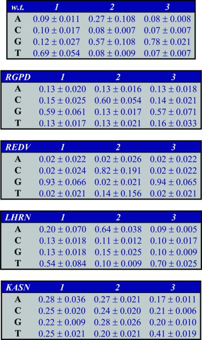
Then we calculate the replica-specific BAMs for each protein, using the probabilities. Initially, we calculate the BAMs assuming that all three base positions are independent (mononucleotide BAMs). For a particular protein, the mononucleotide BAM of replica k is represented by 12 weights, P k ij, where i is the base position (i = 1,2,3) and j is the nucleotide type (j = A,C,G,T). The weights correspond to the probabilities of interaction and are determined by summing the corresponding probabilities as defined in equation 1. For example, the parameter that corresponds to A at position 1 is the sum of the probabilities of all sequences of the form ANN. Note that under additivity the sum of the probabilities in each position should be 1.0, hence the number of free parameters needed to be estimated is 9.
In a similar way, we calculate the corresponding dinucleotide BAMs (data not shown). For each data set there are two dinucleotide BAMs. For one of them, model 12*3, the two initial positions are considered ‘linked’, but the last position is considered independent. In the other one, model 1*23, the first position is considered independent and the two last positions are considered ‘linked’. We note that both dinucleotide models contain 18 free parameters, which is twice as many as the mononucleotide BAMs. One can also make a first-order Markov model (4), where the probability of a base at each position depends on the previous base (27 or 36 parameters depending on how the first variable base is treated), but that model was not used in the comparisons of the previous paper (4) so we do not include it here.
The above procedure results in nine replica-specific weight matrices for each of the mono and dinucleotide BAMs of each of the proteins (five matrices in the case of the KASN protein). The average values and the standard deviations of the matrices of the mononucleotide BAMs are presented in Table 1.
Table 1. The mononucleotide BAMs for the five proteins.
Correlation between measured probability data and predictions of the best additive model
Having estimated the parameters for the mono- and dinucleotide BAMs for each of the replicas of a protein, we calculate (back) the probability of interaction of any given composite trinucleotide target under the particular additive model. To calculate the predicted probabilities for the trinucleotides under each replica-specific model, we multiply the corresponding position-specific probabilities of the independent positions of the target positions of this model. For the mononucleotide BAMs, the positions of the matrix correspond to the positions in the DNA target. For the dinucleotide BAMs, there are two independent ‘positions’: one with 16 possible states (all 16 dinucleotide combinations for the two ‘linked’ DNA positions) and one with four possible states (the independent DNA position).
Each of the weight matrices that constitutes a replica-specific BAM is used to calculate the predicted probabilities of binding for the 64 trinucleotides. These probabilities are the product of the probabilities of the corresponding bases or dinucleotides in the independent positions (three independent positions for the mononucleotide BAMs and two for the dinucleotide ones). The nine sets of (replica-specific) predicted probabilities of a particular model of a protein (except KASN which has only five sets per model) are averaged and these average values are compared with the average normalised measured K A values using the correlation coefficient. The normalisation of the measured data ensures that the replica-specific values will correspond to probabilities (before averaging them). The calculated correlation coefficients for all proteins are presented in Table 2. In the previous study (4), the average measured K A values were not normalised, which accounts for the slight differences in correlations reported here from those reported previously.
Table 2. Correlation coefficients of the normalised measured K A values compared with the predicted probabilities of the corresponding BAMs.
| Correlation coefficients | |||
|---|---|---|---|
| Zif268 variant | 1*2*3 | 12*3 | 1*23 |
| Wild-type | 0.973 | 0.986 | 0.987 |
| RGPD | 0.883 | 0.942 | 0.941 |
| REDV | 0.999 | 0.999 | 0.999 |
| LRHN | 0.927 | 0.978 | 0.956 |
| KASN | 0.695 | 0.791 | 0.718 |
All calculated values are very similar to the ones reported in Table 1 of the Bulyk et al. paper (4) (see also the legend of Table 2). These data show a very good fit of the experimental values to the ones predicted by the mononucleotide BAMs (0.88 or better for all but the KASN protein). Protein KASN exhibits the weakest correlation (R = 0.695), but this is expected because KASN has low specificity to all DNA targets. All its K A values are <4.7 × 10⁻³ nM–1 and the bases are nearly equiprobable, especially in the first two variable DNA positions (Table 1). Its highest K A value is about 80 times smaller than the highest K A value of the wild-type protein. Moreover, the correlations between the five replicas for the KASN protein have a mean value of only 0.67, while for each of the other four proteins the mean correlation among the nine replicas is between 0.91 and 0.99. In other words, KASN is not only quite non-specific in its binding compared with the other proteins, but the consistency between repeated measurements is also not nearly as high.
In agreement with the previous study, we observe a better performance of the dinucleotide models over the mononucleotide ones. However, the corrected data show that the improvement in correlation coefficient is small. That is, the improvement of the dinucleotide models over the mononucleotide ones for the four proteins that exhibit specific binding is between 0.0 and 0.059. For the KASN protein, the best dinucleotide model differs from the mononucleotide one by 0.096. We also calculate the corresponding _P_-values of the correlation coefficients, using the two tailed Student’s _t_-distribution (8). In all cases, the null hypothesis (i.e. R = 0.0) is rejected at a level of 0.02 (in the case of KASN) or lower.
Models’ comparison
The dinucleotide models are required to fit the data at least as well as the mononucleotide ones because of their extra parameters. In the worst case, the extra parameters would simply be set to zero and the models would fit equally well. But we can ask whether this better fit is significant with the use of an appropriate F-test. Suppose that we have two models, _M_1 and _M_2, that fit some experimental data and that model _M_2 has k parameters more than model _M_1. If we denote by n the number of parameters of model _M_2, the following statistic follows (asymptotically) the F-distribution with k and N – n – 1 degrees of freedom (9):
F = [(D _M_1 – D _M_2)/_k_]/[D _M_2/(N – n – 1)]2
where N is the number of categories of the data and D denotes the deviance (a log-likelihood ratio statistic) of the corresponding models from the observed data. The deviance of each model is two times the relative entropy (9) (see below for definition of relative entropy). The statistic calculated from equation 2 is used to determine the confidence level for rejecting the _H_0 hypothesis that the coefficients of the additional parameters of the model _M_2 are zero.
In our case, _M_1 and _M_2 are the mono- and dinucleotide models, respectively, N = 64 (number of points to fit), n = 18 (number of parameters of the dinucleotide models that are calculated from the data) and k = 9 (additional parameters of the dinucleotide models over the mononucleotide ones). Using this F-statistic we find that for half of the dinucleotide model predictions the improvement over that of the mononucleotide models is not significant at the 0.01 level. In particular, the dinucleotide models that are found to be significantly better than the mononucleotide ones are model 1*23 of the wild-type protein and both dinucleotide models of the RGPD and LRHN proteins. None of the other dinucleotide models is significantly better than the mononucleotide ones even at the 0.05 level.
Figure 1 plots the probabilities from the mono- and the dinucleotide BAMs compared with the measured probabilities. The deviation of each model from the diagonal shows its deviation from a perfect fit to the data. Although the models deviate from the perfect fit to different degrees, they generally present a good fit of an additive, straight line, especially for the high probability states. As expected, the low probability states (i.e. non-specific binding) are ‘clustered’ together in all models and additivity is violated there. We note, though, that by using any cut-off as low as 0.1, and often lower, all models predict the same triplets as high and low probability ones (except in the case of KASN protein where all triplets have probability <0.05). Despite the fact that no additive model fits the measured data perfectly and the fact that the dinucleotide models offer a better fit to the measured data, the mononucleotide additive models are nearly as good as the dinucleotide ones in predicting and ranking the high probability sites.
Figure 1.

Probability plots. The probability distributions of the measured data (abscissas) and the BAM predictions (ordinates) are plotted for the EGR DNA-binding proteins. The predictions are based on additive models under different levels of additivity: blue, red and green marks correspond to the 1*2*3, 12*3 and 1*23 models. Each scatter plot contains all 64 data points, although many data points may coincide. The grey diagonal line represents the ideally best fit of the predictions to the measurements. The scatter plot of protein KASN shows an example of failure of additive models to represent the real data of a non-specific binding protein (note that all probability values, measured and predicted, are <0.05).
Relative entropy and information content: better criteria for comparison
We also compare the observed and predicted normalised average probability distributions of the trinucleotide targets with respect to their relative entropy. The relative entropy is defined as:

where Q and P are the two distributions to be compared (in our case, Q and P will be the probability distributions of the measured data and the additive models, respectively). If the two distributions are similar, especially in the high probability states, then their relative entropy will be close to zero [ (Q || P) ≥ 0 with equality if and only if Q = _P_]. In a recent review (10) we argued that the relative entropy is a more appropriate measure of the goodness-of-fit of the affinity data. The reason is that it is most important for a model to be accurate in the high probability states. When the specificity of the protein decreases (and the affinity is mainly determined by the non-specific contacts), its precise prediction is of limited value. In fact, relative entropy measures the difference between the true and predicted values of the free energy of the entire system (1,11) (see below). Unfortunately, at the time that the review was written, the data of Bulyk et al. (4) were not available, so we could only provide a fictitious example to illustrate the point.
Relative entropy is a special case of a log-likelihood ratio, which measures which of two probability distributions is a better fit to a particular dataset and by how much. Given a dataset D = (_d_1,_d_2,…,d k) and two probability distributions Q and P, the likelihood ratio of generating the data from the two distributions is:

If we replace the observed data d i by a frequency distribution f i = d i /N (where N is the total number of observations, i.e. the sample size) and take the logarithm, then we get the log-likelihood ratio:

This is the general form of the log-likelihood ratio which serves to measure how much better (or worse) any probability distribution fits a particular dataset than any other distribution. The probability distribution with the best fit, the maximum likelihood distribution, is q i = f i. Therefore the relative entropy between the maximum likelihood distribution, F, and any other distribution, P, is:
H(F || P) = (1/N) · LLR(F,P | D)6
The relative entropy also measures the difference in free energy of the system compared with that predicted from the model. The logarithms of the probabilities for binding (or, equivalently, the K _A_s) are proportional to the binding energies. If E i is the true binding energy to site i (from the measured distribution F) and Ê i is the predicted energy (from the distribution of the additive model P), then from equations 5 and 6 we have:

That is, the relative entropy is proportional to the average (taken over all of the bound sites) of the discrepancy between the true and predicted binding energies. Small values indicate that the system as a whole is well approximated by the model. If we consider all the models of a particular type (e.g. all mononucleotide models or all dinucleotide models, etc.), then the one with the lowest relative entropy is the one with the maximum likelihood. The maximum likelihood model is what we call BAM in this study.
We can use the relative entropy to compare a true distribution with a model of that distribution in order to measure how well the model approximates the true distribution. Table 3 lists the relative entropies of the mono- and dinucleotide models compared with the true trinucleotide distribution for the EGR proteins. Except for the protein KASN, which shows very little specificity, the relative entropy values are small compared with the information content (see below), which implies that most of the information in the binding sites is captured by the additive models. Furthermore, in most cases the reduction of relative entropy for dinucleotide models is modest, indicating that they offer only a small improvement to the fit.
Table 3. Relative entropies of the predicted versus measured probability distributions for the mono- and dinucleotide models.
| Relative entropy | |||
|---|---|---|---|
| Zif268 variant | 1*2*3 | 12*3 | 1*23 |
| Wild-type | 0.244 | 0.188 | 0.137 |
| RGPD | 0.336 | 0.192 | 0.213 |
| REDV | 0.136 | 0.096 | 0.098 |
| LRHN | 0.245 | 0.139 | 0.136 |
| KASN | 0.076 | 0.057 | 0.070 |
A special case of relative entropy is the information content, which is defined as the relative entropy of a distribution over the background distribution:

where P* is the background (reference) distribution and the distribution from which we calculate the information content. We note that in our case the information content of a distribution differs from its entropy by a constant because P* is constant (equiprobable background).
In the past, we have defined the information content of a DNA-binding protein as the relative entropy between its observed sequence frequencies and the genomic sequence frequencies (1,12). The higher the information content the more specific the protein is and less frequent its binding sites in the genome. In pattern recognition methods that attempt to identify the transcription factor binding sites in sets of co-regulated genes, information content can be used as the criterion to rank different alignments of sites and pick the most significant (13,14). In fact, information content does not give an accurate _P_-value by itself, but it can be used to estimate the _P_-value and E-value of an alignment (15). Information content is usually measured using the observed frequencies at each position in the binding site and the genomic base composition, hence assuming additivity between the positions. But it can be done at any level, from the individual bases to dinucleotides to the complete binding sites. Table 4 lists the information content for each of the five EGR proteins as determined from the mono-, di- and trinucleotide level distributions. The trinucleotide information content is based on the measured probability distribution over all 64 trinucleotides. These data show that the information content based on mononucleotides is usually fairly close to that based on the complete binding sites.
Table 4. The information content of the various distributions.
| Information content | ||||
|---|---|---|---|---|
| Zif268 variant | 1*2*3 | 12*3 | 1*23 | measured |
| Wild-type | 1.35 | 1.40 | 1.45 | 1.59 |
| RGPD | 0.77 | 0.93 | 0.91 | 1.13 |
| REDV | 2.94 | 3.00 | 3.00 | 3.14 |
| LRHN | 0.99 | 1.10 | 1.10 | 1.24 |
| KASN | 0.07 | 0.09 | 0.08 | 0.15 |
Analysis of the data for the Mnt repressor-operator protein
We also analyse the data presented by Man and Stormo (3) (see Fig. 2), using the same methods. Our results agree with the authors’ that these data show a violation of additivity at positions 16 and 17. However, the correlation coefficient of their calculated probabilities over all dinucleotides and the ones obtained under additivity is 0.95 (P = 0.01). Moreover, the relative entropy is 0.06, which shows that the BAM does not deviate much from the real data in this case either. The information content of the distribution of the BAM for this protein is 0.62 and for the distribution of the real data is 0.68.
Figure 2.

A graphical representation of the non-independent effect of positions 16 and 17 of the Mnt DNA binding site. In the left graph, the probabilities based on the measured K A values are plotted against the 1*2 additive model. In the case of Mnt, the deviation from additivity in the high probability states is higher than that of Figure 1. However, the right graph plots the two probability distributions by dinucleotide target and shows that the additive model is in pretty good agreement with the measured data. These graphs are based on the data reported in the study of Man and Stormo (3).
DISCUSSION
The data published by Bulyk et al. (4) gives us the rare opportunity to assess the significance of the additivity hypothesis in modelling protein–DNA interactions. From that study and the one by Man and Stormo (3) it has become clear that the BAM cannot generally provide a perfect fit for the data. However, we find that in most of the studied cases, the additive models constitute very good approximations of the measured probabilities.
The extent of this goodness-of-fit varies from protein to protein. The mononucleotide BAM for the protein REDV, for example, shows a nearly perfect correlation with the experimental data. In the case of protein KASN, though, we find a much poorer fit, probably due to the low specificity of this protein. We also find strong correlations between the mononucleotide BAMs and the measured data for the other three EGR proteins as well as for the Mnt protein. When dinucleotide models are considered for the EGR proteins, we find that the improvement of the correlation coefficient is very low (<0.1). The F-test shows that this small improvement is statistically significant at the 0.01 level for half of the dinucleotide models.
Optimising energy versus optimising probability
There are other approaches for finding and testing additive models to quantitative data. Stormo et al. (16) used multiple regression to obtain parameters for mono- and dinucleotide models for several different types of data. They showed that in one case a mononucleotide model was quite good, but in another a dinucleotide model was needed for an adequate fit. In a third case neither model provided a good fit to the data. Recently, Lee et al. (17) performed a multiple regression analysis of the data from Bulyk et al. (4) that we have analysed in this paper. Their conclusions are quite different from ours because of the criteria used for determining the ‘best fit’ model, and measuring how good the fit is. As described in detail in Stormo et al. and Lee et al. (16,17), linear multiple regression finds the coefficients for a set of features that minimise the difference between the observed and the predicted values. The features are the mono- and dinucleotides (and higher levels can be treated in the same way) that occur in the different positions in the binding sites. If these contribute independently to the binding probability then those features should contribute additively to the logarithm of the binding probability. Essentially the model assumes that each feature contributes some binding energy and those contributions sum to give the total binding energy, which is proportional to the logarithm of the binding probability. Analysis of variance methods can be used to compare different models to determine which is the best and which features contribute significantly to the fit. Lee et al. (17) find that all of the higher level models provide significant improvements over the mononucleotide model.
Our conclusions differ because we use a very different criterion for the best fit. Consider a true probability distribution, Q, and a model that provides a predicted distribution, P. In the regression method of Stormo et al. and Lee et al. (16,17) the measure of fitness is the sum of the squares of the differences between the logarithms of the probabilities for all of the data points:

The best model is that with a minimum of M(Q,P). Note that the main difference between this criterion and relative entropy is that all of the sites contribute equally to the measure of fitness, whereas relative entropy gives more weight to the more probable binding sites. A weighted multiple regression could be performed, but it was not included in the models presented in the previous two studies (16,17). Relative entropy is also closely related to χ2 (9), another fitness measure:

where N is the sample size. The best model by the criterion of minimum relative entropy is the one that maximises the likelihood of the data.
Both the regression method and the maximum likelihood method are standard statistical approaches for modelling quantitative data and neither should be considered ‘right’ or ‘wrong’. They simply measure different things and use different criteria for ‘best fit’. The differences are clear upon examining equations 9 and 10. Multiple regression, as applied in Stormo et al. and Lee et al. (16,17), minimises the squared differences in the logarithms of the binding probabilities (equivalent to minimising the squared difference of the binding energies), and does so without weighting any sites more than others. The relative entropy approach obtains the maximum likelihood model, which naturally emphasises the high probability sites. Equation 7 also shows that relative entropy measures the average discrepancy between the measured and predicted binding energies.
Figure 3 compares the two approaches using the EGR1 binding data (4). Figure 3A shows the fit of the mononucleotide models, using both approaches, to the logarithms of the binding probabilities. The regression model (RM) is a better fit in this plot, primarily because its spread at the high values (i.e. the low affinity sites) is much less than that of the BAM. This comes at the expense of having a much worse fit to the low energy (high affinity) sites, but because there are many more low affinity sites than high affinity ones, the overall fit of the RM is better in this plot. Figure 3B shows the fit to the probability data. Now the BAM is the much better fit. In this plot both models appear to fit the low probability sites equally well, because they are all clustered together in a small area in the corner of the plot. But only the BAM gives a good fit to the high probability sites and RM is far off. We do not show RMs for the dinucleotide models that fit better, because our main point is that even mononucleotide models can give quite good fits by the criterion of minimum relative entropy (or maximum likelihood). Because low affinity interactions are largely due to non-specific contacts we do not expect them to be determined by additive contributions from the bases. Furthermore, for purposes of predicting new binding sites in a genome sequence, we are primarily interested in those sites with high probabilities of binding. Those are also the sites that have the dominant effect on the free energy of the entire system. The relative entropy method emphasises the above criteria, which we consider to be most important for prediction of DNA binding sites. Thus, we use this method to obtain what we call the BAMs.
Figure 3.

Probability and log-probability plots. Scatter plots of the negative logarithms (A) and the predicted binding probabilities (B) for the mononucleotide models that provide ‘best fit’ to the data, according to different criteria. The BAM that we calculate in this paper minimises the squared difference between the predicted and the measured probabilities in the data. The regression model (RM) minimises the squared difference between the predicted and the measured log-probabilities of the data (equivalent to energies). This model was calculated using the BLSS package (42) on the normalised average K A values of the wild-type EGR protein. Methods for calculating such regression models also exist in the literature (16,17). The two plots show that BAM is better than RM at predicting the high probability targets, whereas RM better fits the high log-probability ones (equivalent to the high energies). The diagonals (straight lines) correspond to the measured values.
Advantages of the additive models
There are two types of advantage in using additive models. The first is the computational performance in the search for binding sites of a protein. With fewer parameters, the additive models can search the sequence sets faster. In a simple implementation, a dinucleotide model has four times as many parameters as a mononucleotide matrix and so searches could take four times as long. However, this is not the most important advantage of the additive models. Faster algorithm implementations can be developed. For example, since searches usually employ a threshold score, and identify all sites above the cut-off, it is easy to pre-compute the set of all sequences that exceed the threshold and search for them simultaneously using finite automata (18). Even using simple search methods, the speed advantage may not be significant in many cases, and it may be worth the extra time required to have more accurate predictions.
The second advantage is likely to be more important in practice, and that is the amount of data required to estimate accurately the extra parameters of the more complex models. The number of parameters increases by a factor of four for each increase in the level of the model of the DNA target; for instance, from mononucleotides to dinucleotides, or dinucleotides to trinucleotides. Collecting the extra quantitative affinity data by conventional means would be laborious and expensive, but new high throughput methods can collect much more data efficiently. The array based method of Bulyk et al. (4,5) can provide quantitative binding data for many individual sites simultaneously. For long binding sites, such as 10 bp zinc-finger sites, all possible sites (>106) cannot be included on the array, as it was for all 64 triplets interacting with the middle finger. But a sufficiently large number of target sites can be included such that accurate high-level models will be obtainable. A different approach, combining in vitro selection from pools of randomised oligonucleotides (i.e. SELEX), followed by quantitative, multiple fluorescence, relative affinity assays (3) can return many binding affinity measurements in a single gel. Because the SELEX step in the procedure returns those sites with the highest affinity (the actual number depending on how many rounds of selection are performed and how many selected sites are sequenced), determining their relative affinities will usually be sufficient to obtain accurate mononucleotide models as well as dinucleotide models for important, non-additive interactions.
Nevertheless, the most common method of estimating binding site models for DNA-binding proteins is likely to remain statistical analyses of known and putative binding sites. Given an alignment of known binding sites, simple log-odds weight matrices (reviewed in 1) provide additive mononucleotide models for the specificity of the protein that can be effective in searching for new sites even if based on only a few, 10–20, known sites. Of course, more known sites will provide more accurate parameter estimates, but it is rare to have enough sites to provide accurate estimates of the four times more parameters in a dinucleotide model. Occasionally there is a sufficient number of examples to build higher-level models, which can be useful. Zhang and Marr (19) made a dinucleotide weight matrix for splice sites and showed that it had a small improvement in the accuracy of predicting splice sites in genomic DNA. Burge and Karlin (20), in the program GenScan, use a more complicated non-additive model for splice site prediction. That model is based on a decision tree that builds separate weight matrices depending on the base occurrences at specific positions. While that model has only a small improvement in the prediction of individual splice sites, it helps significantly in the prediction of complete gene structures. In those cases the extra parameters could be estimated accurately because there are many hundreds (19) or thousands (20) of known splice sites. For most transcription factors the number of known sites is less than one hundred, and often only a few (21). In most such cases one is limited in practice to simple additive models. But the results presented here show that, even in cases where additivity is clearly violated, additive models can still be effective search tools.
Another currently common method for estimating binding site patterns is to employ pattern discovery algorithms on sets of promoter regions from co-regulated genes. A variety of algorithms exist that try to discover the binding sites responsible for the co-regulation (reviewed in 1). Many of those methods model the binding sites as weight matrices, or additive models, and attempt to find the alignment of sites with the maximum information content, or some related likelihood measure. Example algorithms include greedy (13,15), expectation-maximization (22,23) and Gibbs’ sampling (14,24–26). It would be possible to modify those algorithms to use dinucleotide, or even higher-level, models for the interactions, but it is unlikely that will improve their performance, which is already quite good. In most cases these methods are able to identify known binding sites from the appropriate collections of co-regulated promoters. They tend to fail, and this has been examined most carefully on simulated data (15,27,28), when the sites themselves have such low information content, and/or the promoter regions that are being searched are so long, that there is a high probability of finding a spurious alignment of sites with equal or greater information content by chance. The fact that the higher-level models have slightly increased information content might make them more easily identified. However, the extra parameters will also increase the information content obtainable by chance. Because the number of parameters increases by almost four at each higher level, and the amount of information gained (at least in the examples examined so far) is a small fraction of the total, the higher-level models may actually perform worse than the simple additive ones. In cases where there are very dramatic non-additive effects, and much of the total information is lost in mononucleotide models, it would be effective to use higher-level models. We know of no examples like that [except for RNA binding sites where the secondary structure is important for the binding (29)] and hence we expect that the simple models will remain the most useful for finding common binding sites in promoter regions. Of course, once the sites are identified and aligned, higher order information may be extracted from them and used to search for new sites with, perhaps, some improvement in accuracy.
Models for a DNA–protein recognition ‘code’ typically use the additivity assumption. There are a number of approaches that have been followed in the development of such ‘codes’. In the most simple one, the model consists of a list of observed base–amino acid contacts. The contacts catalogued in this way are usually family-specific and position dependent. A protein–DNA pair is evaluated for the potentials of interaction with respect to the number of ‘valid’ contacts that the model can predict (i.e. the ones included in the list). This is the qualitative model that was first presented by Choo and Klug (30,31) and later by Pabo and co-workers (32–34). A different type of modelling, the quantitative models, assign a score to each contact that can be used to rank all possible targets. The score is obtained from a weight matrix that represents the single base–amino acid potentials of the interactions. Quantitative models have been developed by several groups (35–41) and their main differences are in the way that they estimate the base–amino acid potentials.
In general, these models assume that the base–amino acid interactions are energetically additive. The additivity assumption is applied to both the protein and the DNA. In this paper we have shown that assuming additivity between the positions in the DNA binding sites is a reasonable approximation, at least for the cases that have been carefully measured. There is much less data about additivity on the protein, whether the effects of changing two amino acids can be well approximated by the sum of their individual effects. The fact that reasonably good predictive models can be obtained from such an assumption, at least for some proteins (41), provides hope that simple models will be useful recognition codes. If not, the amount of data needed to estimate the parameters will grow enormously. Increasing from a mononucleotide to a dinucleotide model increases the number of parameters by a factor of four, but increasing from a mono-amino acid model to a di-amino acid model increases the parameter number by a factor of 20. Furthermore, the simple model with one amino acid interacting with one base pair has a total of 80 parameters, one for each possible combination. But if we need to model all dinucleotides interacting with all di-amino acids, the number of parameters grows to 6400 per interaction. In such cases the additivity assumption greatly reduces the number of parameters to be estimated, and therefore the amount of data needed. But the real issue is whether such models provide reasonable approximations to reality. They need not be exactly correct to be useful, merely accurate enough to provide specific hypotheses that can be tested in order to validate or refine the models and their predictions.
Acknowledgments
ACKNOWLEDGEMENTS
This work was supported by NIH Grants HG00249 and GM28755 to G.D.S. M.L.B. was partially funded by an Informatics Research Starter Grant from the PhRMA Foundation.
REFERENCES
- 1.Stormo G. (2000) DNA binding sites: representation and discovery. Bioinformatics, 16, 16–23. [DOI] [PubMed] [Google Scholar]
- 2.Stormo G. (1990) Consensus patterns in DNA. Methods Enzymol., 183, 211–221. [DOI] [PubMed] [Google Scholar]
- 3.Man T.-K. and Stormo,G. (2001) Non-independence of Mnt repressor-operator interaction determined by a new quantitative multiple fluorescence relative affinity (QuMFRA) assay. Nucleic Acids Res., 15, 2471–2478. [DOI] [PMC free article] [PubMed] [Google Scholar]
- 4.Bulyk M., Johnson,P. and Church,G. (2002) Nucleotides of transcription factor binding sites exert inter-dependent effects on the binding affinities of transcription factors. Nucleic Acids Res., 30, 1255–1261. [DOI] [PMC free article] [PubMed] [Google Scholar]
- 5.Bulyk M., Huang,X., Choo,Y. and Church,G. (2001) Exploring the DNA-binding specificities of zinc fingers with DNA microarrays. Proc. Natl Acad. Sci. USA, 98, 7158–7163. [DOI] [PMC free article] [PubMed] [Google Scholar]
- 6.Pavletich N. and Pabo,C. (1991) Zinc finger-DNA recognition: crystal structure of a Zif268-DNA complex at 2.1 Å. Science, 252, 809–817. [DOI] [PubMed] [Google Scholar]
- 7.Elrod-Erickson M., Rould,M., Nekludova,L. and Pabo,C. (1996) Zif268 protein–DNA complex refined at 1.6 Å: a model system for understanding zinc finger–DNA interactions. Structure, 4, 1171–1180. [DOI] [PubMed] [Google Scholar]
- 8.Sokal R. and Rohlf,F. (1981) Biometry. W.H. Freeman and Company, New York, NY.
- 9.Dobson A. (2002) An Introduction of Generalized Linear Models. Chapman-Hall, Boca Raton, FL.
- 10.Benos P., Lapedes,A. and Stormo,G. (2002) Is there a code for protein–DNA recognition? Probab(ilistical)ly... Bioessays, 24, 66–75. [DOI] [PubMed] [Google Scholar]
- 11.Stormo G. (1998) Information content and free energy in DNA-protein interactions, J. Theor. Biol., 195, 135–137. [DOI] [PubMed] [Google Scholar]
- 12.Schneider T., Stormo,G., Gold,L. and Ehrenfeucht,A. (1986) Information content of binding sites on nucleotide sequences. J. Mol. Biol., 188, 415–431. [DOI] [PubMed] [Google Scholar]
- 13.Stormo G. and Hartzell,G.,III (1989) Identifying protein-binding sites from unaligned DNA fragments. Proc. Natl Acad. Sci. USA, 86, 1183–1187. [DOI] [PMC free article] [PubMed] [Google Scholar]
- 14.Lawrence C., Altschul,S., Boguski,M., Liu,J., Neuwald,A. and Wootton,J. (1993) Detecting subtle sequence signals: a Gibbs sampling strategy for multiple alignment. Science, 262, 208–214. [DOI] [PubMed] [Google Scholar]
- 15.Hertz G. and Stormo,G. (1999) Identifying DNA and protein patterns with statistically significant alignments of multiple sequences. Bioinformatics, 15, 563–577. [DOI] [PubMed] [Google Scholar]
- 16.Stormo G., Schneider,T. and Gold,L. (1986) Quantitative analysis of the relationship between nucleotide sequence and functional activity. Nucleic Acids Res., 14, 6661–6679. [DOI] [PMC free article] [PubMed] [Google Scholar]
- 17.Lee M.-L., Bulyk,M., Whitmore,G. and Church,G. (2002) A statistical model for investigating binding probabilities of DNA nucleotide sequences using microarrays. Biometrics, 58, in press. [DOI] [PubMed] [Google Scholar]
- 18.Cormen T., Leiserson,C. and Rivest,R. (1990) Introduction to Algorithms. MIT Press, Cambridge, MA.
- 19.Zhang M. and Marr,T. (1993) A weight array method for splicing signal analysis. Comput. Appl. Biol. Sci., 9, 499–509. [DOI] [PubMed] [Google Scholar]
- 20.Burge C. and Karlin,S. (1997) Prediction of complete gene structures in human genomic DNA. J. Mol. Biol., 268, 78–94. [DOI] [PubMed] [Google Scholar]
- 21.Wingender E., Chen,X., Fricke,E., Geffers,R., Hehl,R., Liebich,I., Krull,M., Matys,V., Michael,H., Ohnhauser,R., Pruss,M., Schacherer,F., Thiele,S. and Urbach,S. (2001) The TRANSFAC system on gene expression regulation. Nucleic Acids Res., 29, 281–283. [DOI] [PMC free article] [PubMed] [Google Scholar]
- 22.Lawrence C. and Reilly,A. (1990) An expectation maximization (EM) algorithm for the identification and characterization of common sites in unaligned biopolymer sequences. Proteins, 7, 41–51. [DOI] [PubMed] [Google Scholar]
- 23.Bailey T. and Elkan,C. (1994) Fitting a mixture model by expectation maximization to discover motifs in biopolymers. ISMB, 2, 28–36. [PubMed] [Google Scholar]
- 24.Spellman P., Sherlock,G., Zhang,M., Iyer,V., Anders,K., Eisen,M., Brown,P., Botstein,D. and Futcher,B. (1998) Comprehensive identification of cell cycle-regulated genes of the yeast Saccharomyces cerevisiae by microarray hybridisation. Mol. Biol. Cell., 9, 3273–3297. [DOI] [PMC free article] [PubMed] [Google Scholar]
- 25.Roth F., Hughes,J., Estep,P. and Church,G. (1998) Finding DNA regulatory motifs within unaligned noncoding sequences clustered by whole-genome mRNA quantitation. Nat. Biotechnol, 16, 939–945. [DOI] [PubMed] [Google Scholar]
- 26.McCue L., Thompson,W., Carmack,C., Ryan,M., Liu,J., Derbyshire,V. and Lawrence,C. (2001) Phylogenetic footprinting of transcription factor binding sites in proteobacterial genomes. Nucleic Acids Res., 29, 774–782. [DOI] [PMC free article] [PubMed] [Google Scholar]
- 27.Workman C. and Stormo,G. (2000) Modeling regulatory networks with weight matrices. Pac. Symp. Biocomp., 5, 464–475. [DOI] [PubMed] [Google Scholar]
- 28.Buhler J. and Tompa,M. (2002) Finding motifs using random projections. J. Comp. Biol., 9, 225–242. [DOI] [PubMed] [Google Scholar]
- 29.Gorodkin J., Stricklin,S. and Stormo,G. (2001) Discovering common stem-loop motifs in unaligned RNA sequences. Nucleic Acids Res., 29, 2135–2144. [DOI] [PMC free article] [PubMed] [Google Scholar]
- 30.Choo Y. and Klug,A. (1994) Selection of DNA binding sites for zinc fingers using rationally randomized DNA reveals coded interactions. Proc. Natl Acad. Sci. USA, 91, 11168–11172. [DOI] [PMC free article] [PubMed] [Google Scholar]
- 31.Choo Y. and Klug,A. (1997) Physical basis of a protein–DNA recognition code. Curr. Opin. Struct. Biol., 7, 117–125. [DOI] [PubMed] [Google Scholar]
- 32.Greisman H. and Pabo,C. (1997) A general strategy for selecting high-affinity zinc finger proteins for diverse DNA target sites. Science, 275, 657–661. [DOI] [PubMed] [Google Scholar]
- 33.Wolfe S., Greisman,H., Ramm,E. and Pabo,C. (1999) Analysis of zinc fingers optimised via phage display: evaluating the utility of a recognition code. J. Mol. Biol., 285, 1917–1934. [DOI] [PubMed] [Google Scholar]
- 34.Miller J. and Pabo,C. (2001) Rearrangement of side-chains in Zif268 mutant highlights the complexities of zinc-finger DNA recognition. J. Mol. Biol., 313, 309–315. [DOI] [PubMed] [Google Scholar]
- 35.Suzuki M. and Yagi,N. (1994) DNA recognition code of transcription factors in the helix-turn-helix, probe helix, hormone receptor and zinc finger families. Proc. Natl Acad. Sci. USA, 91, 12357–12361. [DOI] [PMC free article] [PubMed] [Google Scholar]
- 36.Suzuki M., Brenner,S., Gerstein,M. and Yagi,N. (1995) DNA recognition code of transcription factors. Protein Eng., 8, 319–328. [DOI] [PubMed] [Google Scholar]
- 37.Mandel-Gutfreund Y. and Margalit,H. (1998) Quantitative parameters for amino acid-base interaction: implications for prediction of protein–DNA binding sites. Nucleic Acids Res., 26, 2306–2312. [DOI] [PMC free article] [PubMed] [Google Scholar]
- 38.Mandel-Gutfreund Y., Baron,A. and Margalit,H. (2001) A structure-based approach for prediction of protein binding sites in gene-upstream regions. Pac. Symp. Biocomp., 6, 139–150. [DOI] [PubMed] [Google Scholar]
- 39.Kono H. and Sarai,A. (1999) Structure-based prediction of DNA target sites by regulatory proteins. Proteins, 35, 114–131. [PubMed] [Google Scholar]
- 40.Benos P., Lapedes,A., Fields,D. and Stormo,G. (2001) SAMIE: statistical algorithm for modeling interaction energies. Pac. Symp. Biocomp., 6, 115–126. [DOI] [PubMed] [Google Scholar]
- 41.Benos P., Lapedes,A. and Stormo,G. (2002) Probabilistic code for DNA recognition by proteins of the EGR–family. J. Mol. Biol., in press. [DOI] [PubMed] [Google Scholar]
- 42.Abrahams D., and Risszrdi,F. (1988) BLSS: the Berkeley Interactive Statistical System. W.W. Norton and Co., New York, NY.