What is the extent of prokaryotic diversity? - PubMed (original) (raw)
What is the extent of prokaryotic diversity?
Thomas P Curtis et al. Philos Trans R Soc Lond B Biol Sci. 2006.
Abstract
The extent of microbial diversity is an intrinsically fascinating subject of profound practical importance. The term 'diversity' may allude to the number of taxa or species richness as well as their relative abundance. There is uncertainty about both, primarily because sample sizes are too small. Non-parametric diversity estimators make gross underestimates if used with small sample sizes on unevenly distributed communities. One can make richness estimates over many scales using small samples by assuming a species/taxa-abundance distribution. However, no one knows what the underlying taxa-abundance distributions are for bacterial communities. Latterly, diversity has been estimated by fitting data from gene clone libraries and extrapolating from this to taxa-abundance curves to estimate richness. However, since sample sizes are small, we cannot be sure that such samples are representative of the community from which they were drawn. It is however possible to formulate, and calibrate, models that predict the diversity of local communities and of samples drawn from that local community. The calibration of such models suggests that migration rates are small and decrease as the community gets larger. The preliminary predictions of the model are qualitatively consistent with the patterns seen in clone libraries in 'real life'. The validation of this model is also confounded by small sample sizes. However, if such models were properly validated, they could form invaluable tools for the prediction of microbial diversity and a basis for the systematic exploration of microbial diversity on the planet.
Figures
Figure 1
Non-parametric methods must be used with caution when sample sizes are small. The sample sizes required to correctly characterize a sample with a diversity (i.e. richness) of 5000, undertaking a complete census, a 95% census or using non-parametric methods (Chao 1 and ACE). Note that if the diversity is uniform, non-parametric estimators are very efficient. However, if the diversity is lognormally distributed, then a very large sample is required to obtain the correct answer. The simulations are described in more detail elsewhere (Schloss & Handelsman in press).
Figure 2
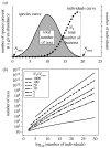
A ‘quick and dirty’ way to estimate diversity by assuming a distribution. (a) The total number of taxa in a community with a lognormal species abundance curve is simply the area under that curve (called the species curve). The individuals curve is the number of species at each abundance (the species curve) multiplied by their abundance (the _x_-axis). There is therefore a mathematical relationship between the area under a species area curve, the number of individuals _N_T (the area under the individuals curve), and the maximum and the minimum abundance (_N_max and _N_min). (b) The relationship, over 30 orders of magnitude in population size, for various ratios of _N_T/_N_max by assuming that _N_min is equal to one (Curtis et al. 2002). As a rule of thumb, soil has a ratio of 10 and seas and lakes have a ratio of 4. There are about 1030 bacteria in the world (Whitman et al. 1998).
Figure 3
Different distributions are observed in the same environment. Clone libraries of different groups of organisms (Archaea and Bacteria) in the same environment can appear to have radically different distributions. Hypothetical geometric (Archaea) and lognormal (Bacteria) distributions are shown. In this example, the bacterial and archaeal 16S rRNA gene sequences amplified from the same anaerobic digester exhibit very different distributions. Thus, the distribution of species is not likely to be a simple function of the suitability of the environment (data from Godon et al. 1997).
Figure 4
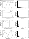
Small samples can be very misleading. To demonstrate the unreliability of small sample sizes, four radically different distributions (on the left) were sampled (200 individuals selected randomly) and the resulting distributions (shown on the right) plotted (Sloan et al. in press). Note that all the sample distributions are superficially alike.
Figure 5
A schematic of the model used to estimate diversity. When an individual dies in the local community, it is replaced from outside the community with a probability m, or from within the community with a probability 1−m (after Hubbell 2001; Sloan et al. 2006, in press).
Figure 6
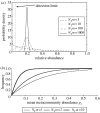
Predictions of the Sloan et al. (2006, in press) model. Probability density functions, ϕ i for the local abundance of a species that makes up 20% of the source community. _m_=1 means the space vacated by every death is filled by an immigrant and the source and local communities are highly coupled. Therefore, ϕ i forms a tight bell-shaped distribution with mean relative abundance 20%. As m drops, the local community becomes increasingly more isolated and the internal neutral dynamics act to increase the skew and variance of the distributions, making low abundances more probable, but increasing the uncertainty or variability. As m continues to drop, the mode of the distribution becomes zero (m<0.04) and the likelihood of the species being absent increases.
Figure 7
How the value of N_T_m and m can be determined. (a) For a given mean source community abundance, the frequency with which an organism is observed is related to N_T_m, the total number of individuals multiplied by the immigration parameter. At high N_T_m values, the local distribution is tightly clustered around the mean meta-community distribution (in this case 0.2). As the N_T_m values drop, the distribution widens and eventually the mode of the curve falls below the detection limit and the organism is no longer observed. There is therefore a relationship between the mean source community abundance N_T_m and the frequency with which an organism is observed. (b) The expected frequency–relative abundance relationships observed in a local community for differing N_T_m values. Thus, for a given dataset, the N_T_m values can be found by fitting a line to these data; where the value of _N_T is known, m can be easily inferred.
Figure 8
Data and theory compared. The theoretical (solid line) and observed (squares or triangles) relationship between the mean relative abundance of taxa and the frequency with which they appear in a population of fixed size. Each of the points represents a different taxon. (a) Clone libraries of different ammonia monooxygenase (AMO) genes at 13 different domestic sewage works, _N_T_m_=1.41 (Wagner & Loy 2002). The triangles represent putative salt tolerant taxa. (b) Clone libraries of 16S rRNA genes from different AOB at six sites from the Humber Estuary, _N_T_m_=14. (c) Clone libraries of 16S rRNA genes from five experimental aquatic microcosms, _N_T_m_=10.3 (Horner-Devine et al. 2003). (d) 16S RNA sequences for 16 different bacterial taxa that are considered to be specific to freshwater environments sampled from 96 different lakes (Zwart et al. 2003), _N_T_m_=1.36. It is interesting to note that though both panels (c) and (d) pertain to lakes, the fit is much better in the larger dataset. This might be for two reasons: first, a larger dataset from larger systems will give a better indication of p i but also because prior to the analysis of (d) we removed data that represented three cyanobacterial lineages, leaving only data from one functional group of putative heterotrophs whereas (c) contains all the bacterial sequences. Other examples and a full description are given in Sloan et al. (2006, in press).
Figure 9
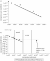
The scaling of immigration with _N_T. From left to right are shown a single cell, through a clone library to a FISH study and a DGGE gel. The solid line is the scaling predicted within a system from the clone library data. The data is shown at (a) a local scale and (b) a global scale, there being approximately 1030 bacteria in the world. It is apparent that a plausible extrapolation of the observed data could bring the rate of immigration below a plausible rate of speciation. This would permit speciation in an open system.
Figure 10
Model predictions are qualitatively consistent with the patterns seen in ‘real life’. A sample of 50 ammonia-oxidizing bacteria (AOB) clones and 500 bacterial clones in one of the wastewater treatment plants featured in figure 9 found taxa diversities of 7 and 202, respectively, in the two samples. Here, we examine the ability of the Sloan et al. model to qualitatively reproduce that finding. We used known _N_T values and, hypothetical source diversities of 200 (for the low source diversity group corresponding with the AOB) and 100 000 (for the high source diversity corresponding with the general bacterial population); immigration parameters were estimated using the extrapolation procedure mentioned in this paper (10−12 for the AOB and 1.5×10⁻¹⁶ for the general bacterial population). (a) Represents the AOB, the diversity is similar to that found in the samples. (b) Represents the high source diversity group, the most abundant members of which are shown in (c) for greater clarity. The clone and local diversity are obviously distinct. Slightly less diversity was found in the model than observed in practice, suggesting some small errors in the source term or the immigration parameter. This is neither proof nor disproof of the model, but an encouraging indication that a more formal validation may be worthwhile undertaking.
Figure 11
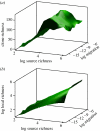
The validation of the model is impossible with small sample sizes. Using the neutral model to simulate the effect of migration and source community diversity in a microbial community of 1018 individuals (e.g. a wastewater treatment plant) on (a) the number of taxa in a library of 500 clones and (b) the true local richness in a community of 1018. The number of taxa in the sample soon plateaus, which means we can infer relatively little about the local or source diversity except that both probably exceed 103 and 104, respectively. Note how the clone library species richness actually dips slightly at higher diversities, probably owing to a change in evenness in the underlying local community.
Similar articles
- Bacterial diversity in aquatic and other environments: what 16S rDNA libraries can tell us.
Kemp PF, Aller JY. Kemp PF, et al. FEMS Microbiol Ecol. 2004 Feb 1;47(2):161-77. doi: 10.1016/S0168-6496(03)00257-5. FEMS Microbiol Ecol. 2004. PMID: 19712332 - Prokaryotic genetic diversity throughout the salinity gradient of a coastal solar saltern.
Benlloch S, López-López A, Casamayor EO, Øvreås L, Goddard V, Daae FL, Smerdon G, Massana R, Joint I, Thingstad F, Pedrós-Alió C, Rodríguez-Valera F. Benlloch S, et al. Environ Microbiol. 2002 Jun;4(6):349-60. doi: 10.1046/j.1462-2920.2002.00306.x. Environ Microbiol. 2002. PMID: 12071980 - Species richness in soil bacterial communities: a proposed approach to overcome sample size bias.
Youssef NH, Elshahed MS. Youssef NH, et al. J Microbiol Methods. 2008 Sep;75(1):86-91. doi: 10.1016/j.mimet.2008.05.009. Epub 2008 May 15. J Microbiol Methods. 2008. PMID: 18585806 - The tragedy of the uncommon: understanding limitations in the analysis of microbial diversity.
Bent SJ, Forney LJ. Bent SJ, et al. ISME J. 2008 Jul;2(7):689-95. doi: 10.1038/ismej.2008.44. Epub 2008 May 8. ISME J. 2008. PMID: 18463690 Review. - The generation and maintenance of diversity in microbial communities.
Fierer N, Lennon JT. Fierer N, et al. Am J Bot. 2011 Mar;98(3):439-48. doi: 10.3732/ajb.1000498. Epub 2011 Feb 17. Am J Bot. 2011. PMID: 21613137 Review.
Cited by
- Planktonic microbes in the Gulf of Maine area.
Li WK, Andersen RA, Gifford DJ, Incze LS, Martin JL, Pilskaln CH, Rooney-Varga JN, Sieracki ME, Wilson WH, Wolff NH. Li WK, et al. PLoS One. 2011;6(6):e20981. doi: 10.1371/journal.pone.0020981. Epub 2011 Jun 15. PLoS One. 2011. PMID: 21698243 Free PMC article. Review. - Development of a prokaryotic universal primer for simultaneous analysis of Bacteria and Archaea using next-generation sequencing.
Takahashi S, Tomita J, Nishioka K, Hisada T, Nishijima M. Takahashi S, et al. PLoS One. 2014 Aug 21;9(8):e105592. doi: 10.1371/journal.pone.0105592. eCollection 2014. PLoS One. 2014. PMID: 25144201 Free PMC article. - Diversity and evolution of class 2 CRISPR-Cas systems.
Shmakov S, Smargon A, Scott D, Cox D, Pyzocha N, Yan W, Abudayyeh OO, Gootenberg JS, Makarova KS, Wolf YI, Severinov K, Zhang F, Koonin EV. Shmakov S, et al. Nat Rev Microbiol. 2017 Mar;15(3):169-182. doi: 10.1038/nrmicro.2016.184. Epub 2017 Jan 23. Nat Rev Microbiol. 2017. PMID: 28111461 Free PMC article. - Ecology and exploration of the rare biosphere.
Lynch MD, Neufeld JD. Lynch MD, et al. Nat Rev Microbiol. 2015 Apr;13(4):217-29. doi: 10.1038/nrmicro3400. Epub 2015 Mar 2. Nat Rev Microbiol. 2015. PMID: 25730701 Review. - Distinct growth strategies of soil bacteria as revealed by large-scale colony tracking.
Ernebjerg M, Kishony R. Ernebjerg M, et al. Appl Environ Microbiol. 2012 Mar;78(5):1345-52. doi: 10.1128/AEM.06585-11. Epub 2011 Dec 22. Appl Environ Microbiol. 2012. PMID: 22194284 Free PMC article.
References
- Bell G. The distribution of abundance in neutral communities. Am. Nat. 2000;155:606–617. doi:10.1086/303345 - DOI - PubMed
- Bell G. Ecology—neutral macroecology. Science. 2001;293:2413–2418. doi:10.1126/science.293.5539.2413 - DOI - PubMed
- Brock T. Prentice-Hall; Englewood Cliffs, NJ: 1966. Principles of microbial ecology.
- Brown J.H. University of Chicago Press; Chicago, IL: 2000. Macroecology.
MeSH terms
LinkOut - more resources
Full Text Sources

