Transfer entropy--a model-free measure of effective connectivity for the neurosciences - PubMed (original) (raw)
Transfer entropy--a model-free measure of effective connectivity for the neurosciences
Raul Vicente et al. J Comput Neurosci. 2011 Feb.
Abstract
Understanding causal relationships, or effective connectivity, between parts of the brain is of utmost importance because a large part of the brain's activity is thought to be internally generated and, hence, quantifying stimulus response relationships alone does not fully describe brain dynamics. Past efforts to determine effective connectivity mostly relied on model based approaches such as Granger causality or dynamic causal modeling. Transfer entropy (TE) is an alternative measure of effective connectivity based on information theory. TE does not require a model of the interaction and is inherently non-linear. We investigated the applicability of TE as a metric in a test for effective connectivity to electrophysiological data based on simulations and magnetoencephalography (MEG) recordings in a simple motor task. In particular, we demonstrate that TE improved the detectability of effective connectivity for non-linear interactions, and for sensor level MEG signals where linear methods are hampered by signal-cross-talk due to volume conduction.
Figures
Fig. 1
Illustration of false positive effective connectivity due to insufficient embedding for delayed interactions. Source signal X drives target signal Y with a delay δ. The internal memory of process X is reflected in the slowly decaying autocorrelation function (top). For the evaluation of TE from Y to X, X is embedded for auto-prediction with d = 3 and τ, as indicated by the dark gray box. The data point of X that is to be predicted with prediction time u is indicated by the star shaped symbol. Data points used for auto-prediction are indicated by filled circles on signal X. Data points used for cross-prediction from Y to X are indicated by filled circles on signal Y. Due to the delayed interaction from X to Y information about X earlier than the embedding time gets transferred from X to Y where it gets included in the embedding (open circle). Y contains information the history of X that is useful for predicting X (see open circle, autocorrelation curve) but not contained in the embedding used on X. Hence, inclusion of Y will improve the prediction of X and false positive effective connectivity is found. Introducing a larger embedding dimension or or larger embedding delay, incorporates this information into the embedding of X. Examples of this effect can be found in Tables 1 and 2
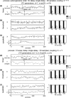
Fig. 2
Detection of effective connectivity by TE for two unidirectionally coupled signals (X →Y). (a–c) Signals generated from an autoregressive order ten process and coupled via (a) linear, (b) threshold, and (c) quadratic coupling. (d–f) Signals generated with dynamics of a 1/f noise process and coupled via (d) linear, (e) threshold, and (f) quadratic coupling. A single interaction delay of 20 samples was used. Time courses of source (X) and target (Y) signals on the left and results of permutation testing for a varying number of trials (15, 30, 60, 120) on the right. Black bars indicate (1-p) values for coupling X →Y (true coupling direction), gray bars indicate values of (1-p) for coupling Y →X. The dashed line corresponds to significant effective connectivity (p < 0.05)
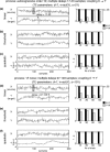
Fig. 3
Detection of effective connectivity by TE for two unidirectionally coupled time series (X →Y) with a range of coupling delays as indicated by the shaded boxes in (a) and (d). (a–c) autoregressive order ten processes; interaction delays 17–23 samples. (a) Linear interaction, (b) threshold coupling, and (c) quadratic coupling. (d–f) 1/f processes; interaction delays 97–103 samples. (d) Linear interaction, (e) threshold coupling, and (f) quadratic coupling. Time series are plotted on the left, results of permutation testing for different numbers of simulated trials (15, 30, 60, 120) on the right. Black bars indicate values of (1-p) for coupling X →Y (true coupling direction), gray bars indicate values of (1-p) for coupling Y →X. The dashed line corresponds to significant effective connectivity (p < 0.05)
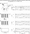
Fig. 4
Simulation results for linearly mixed measurements (X ε, Y ε ) of two unidirectionally and linearly coupled underlying source signals (X →Y). (a) Mixing model and original autoregressive source time courses X, Y. (b–d) Effective connectivity between sensor-level signals X ε, Y ε. Left statistics of permutation tests of TE values for the original sensor level data against trial-shuffled surrogate data after application of the additional time-shift test. The plots contain values of (1-p) in dependence of the number of investigated number of trials. Black bars indicate values for the effective connectivity from the sensor dominated by the driving source signal (X ε) to the sensor dominated by the receiving source signal (Y ε). Light grey bars indicate the reverse direction of effective connectivity. The dashed line corresponds to siginificant effective connectivity (p < 0.05). Right time- courses of signals X ε and Y ε for a single trial
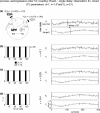
Fig. 5
Simulation results for linearly mixed measurements (X ε, Y ε ) of two unidirectionally coupled underlying source signals (X →Y) coupled via a threshold function. (a) Mixing model and original autoregressive source time courses X, Y. (b–d) Effective connectivity between sensor-level signals X ε, Y ε. Left statistics of permutation tests of TE values for the original sensor level data against trial-shuffled surrogate data after application of the additional time-shift test. Black bars indicate values for the effective connectivity from the sensor dominated by the driving source signal (X ε) to the sensor dominated by the receiving source signal (Y ε). Light grey bars indicate the reverse direction of effective connectivity. The dashed line corresponds to siginificant effective connectivity (p < 0.05). Right time-courses of signals X ε and Y ε for a single trial
Fig. 6
False positive rates for the detection of effective connectivity when observing one source via two EEG or MEG sensors. (a) Signal generation by an autoregressive order ten process X(t) and simultaneous observation of this source signal on two sensor signals X ε, Y ε. One of the signals is a copy of the source signal (X ε (t) = X(t)); the other, (Y ε), is dampened by a factor of (1 − ε) and corrupted by white noise εη. (b) Resulting signal time courses for the source signal X(t) and the observed sensor signals Y ε for different values of ε. (c) False positive detection rate for effective connectivity from the noise free sensor signal X ε to the noise corrupted signal Y ε before (dashed line) and after (solid line) the additional time-shift test for instantaneous mixing. In accordance with (Nolte et al. 2008) TE without the additional test yields a certain amount of false positive results. (d) False positive detection rate for effective connectivity from the noise corrupted signal Y ε to the noise free sensor signal X ε. Lines as in (c). No false positives were observed after the additional time shifting test
Fig. 7
Neuromagnetic fields in a finger lifting task. (a) Single-trial raw traces of magnetic fields (thin line) measured by two MEG sensors over left (MLT24) and right (MRT24) motor cortex (also compare (d) for the position of these sensors). In this trial the right finger was lifted. (b) Corresponding single trial EMG traces obtained from the left (EMG L) and right (EMG R) forearm. Time ‘0’ indicates the sample when the light barrier switch detected the finger lift. (c) Topography of magnetic fields averaged over trials at −50 ms before the registration of a right index finger lift. Note the dipolar pattern over left central cortex. (d) Layout of the MEG sensors. Sensors used for analysis of effective connectivity are indicated by solid circles. Lines with arrowheads indicate the investigated connections
Fig. 8
Differences in effective connectivity (EC) between lifting of the right (RFL) and left index finger (LFL) for subject 1 (left) and subject 2 (right). The investigated frequency band was 5–29 Hz encompassing the μ and β rhythms, and avoiding 50 Hz contamination. Red lines indicate links where effective connectivity as quantified by TE was significantly larger for lifting of the right index finger, compared to left. Blue lines indicate links where effective connectivity as quantified by TE was significantly larger for lifting of the left index finger, compared to right. Connectivity from contra- and ipsilateral motor cortices to muscles (EMG L, EMG R) of the moved finger is stronger than to the passive finger
Similar articles
- Quantification of effective connectivity in the brain using a measure of directed information.
Liu Y, Aviyente S. Liu Y, et al. Comput Math Methods Med. 2012;2012:635103. doi: 10.1155/2012/635103. Epub 2012 May 16. Comput Math Methods Med. 2012. PMID: 22675401 Free PMC article. - Phase transfer entropy: a novel phase-based measure for directed connectivity in networks coupled by oscillatory interactions.
Lobier M, Siebenhühner F, Palva S, Palva JM. Lobier M, et al. Neuroimage. 2014 Jan 15;85 Pt 2:853-72. doi: 10.1016/j.neuroimage.2013.08.056. Epub 2013 Sep 2. Neuroimage. 2014. PMID: 24007803 - Nonlinear effective connectivity measure based on adaptive Neuro Fuzzy Inference System and Granger Causality.
Farokhzadi M, Hossein-Zadeh GA, Soltanian-Zadeh H. Farokhzadi M, et al. Neuroimage. 2018 Nov 1;181:382-394. doi: 10.1016/j.neuroimage.2018.07.024. Epub 2018 Jul 19. Neuroimage. 2018. PMID: 30010006 - Investigating effective brain connectivity from fMRI data: past findings and current issues with reference to Granger causality analysis.
Deshpande G, Hu X. Deshpande G, et al. Brain Connect. 2012;2(5):235-45. doi: 10.1089/brain.2012.0091. Brain Connect. 2012. PMID: 23016794 Free PMC article. Review. - Analysing connectivity with Granger causality and dynamic causal modelling.
Friston K, Moran R, Seth AK. Friston K, et al. Curr Opin Neurobiol. 2013 Apr;23(2):172-8. doi: 10.1016/j.conb.2012.11.010. Epub 2012 Dec 21. Curr Opin Neurobiol. 2013. PMID: 23265964 Free PMC article. Review.
Cited by
- Entropy-based analysis and bioinformatics-inspired integration of global economic information transfer.
Kim J, Kim G, An S, Kwon YK, Yoon S. Kim J, et al. PLoS One. 2013;8(1):e51986. doi: 10.1371/journal.pone.0051986. Epub 2013 Jan 2. PLoS One. 2013. PMID: 23300959 Free PMC article. - Measuring inter- and intra-individual differences in visual scan patterns in a driving simulator experiment using active information storage.
Wiebel-Herboth CB, Krüger M, Wollstadt P. Wiebel-Herboth CB, et al. PLoS One. 2021 Mar 18;16(3):e0248166. doi: 10.1371/journal.pone.0248166. eCollection 2021. PLoS One. 2021. PMID: 33735199 Free PMC article. - Phase-amplitude coupling at the organism level: The amplitude of spontaneous alpha rhythm fluctuations varies with the phase of the infra-slow gastric basal rhythm.
Richter CG, Babo-Rebelo M, Schwartz D, Tallon-Baudry C. Richter CG, et al. Neuroimage. 2017 Feb 1;146:951-958. doi: 10.1016/j.neuroimage.2016.08.043. Epub 2016 Aug 21. Neuroimage. 2017. PMID: 27557620 Free PMC article. - Revealing the structure of information flows discriminates similar animal social behaviors.
Valentini G, Mizumoto N, Pratt SC, Pavlic TP, Walker SI. Valentini G, et al. Elife. 2020 Jul 30;9:e55395. doi: 10.7554/eLife.55395. Elife. 2020. PMID: 32730203 Free PMC article. - Successful Object Encoding Induces Increased Directed Connectivity in Presymptomatic Early-Onset Alzheimer's Disease.
Ochoa JF, Alonso JF, Duque JE, Tobón CA, Mañanas MA, Lopera F, Hernández AM. Ochoa JF, et al. J Alzheimers Dis. 2017;55(3):1195-1205. doi: 10.3233/JAD-160803. J Alzheimers Dis. 2017. PMID: 27792014 Free PMC article.
References
- Cao L. Practical method for determining the minimum embedding dimension of a scalar time series. Physica, A, 1997;110:43–50.
- Cormen, T., Leiserson, C., Rivest, R., & Stein, C. (2001). Introduction to algorithms. MIT Press and McGraw-Hill.
- Donoghue JP, Sanes JN, Hatsopoulos NG, Gal G. Neural discharge and local field potential oscillations in primate motor cortex during voluntary movements. Journal of Neurophysiology. 1998;79(1):159–173. - PubMed
Publication types
MeSH terms
LinkOut - more resources
Full Text Sources
Other Literature Sources
Miscellaneous


