{\em Pretty Damn Quick} Performance Analyzer (original) (raw)
PDQ: {\em Pretty Damn Quick} Performance Analyzer
From a performance standpoint, a modern computer system can be thought of as a directed graph of individual buffers where requests may wait for service at some computational resource, e.g., a CPU processor. Since a buffer is just a queue, all computer systems can be represented as a directed graph of queues. The directed arcs represent flows between different queueing resources. PDQ computes the performance metrics of such a graph. A directed graph of queues is generally referred to as a queueing network model.
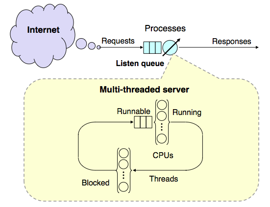
Queueing network model of a multi-threaded web service running on a multicore server
1 What is PDQ?
PDQ (Pretty Damn Quick) a queueing network performance analyzer that comes as:
- a free open source software package
- with an online user manual PDQ is a standalone application that is closely associated with the books Analyzing Computer System Performance with Perl::PDQ(Springer 1st edn. 2005, 2nd edn. 2011) and_The Practical Performance Analyst_(McGraw-Hill 1998, iUniverse.com Press 2000) and Guerrilla training classes. PDQ uses queue-theoretic paradigms to represent and solve all kinds of modern computer systems. Computer system resources (whether hardware and software) are represented by queues (more formally, a queueing network-not to be confused with a data network-which could be a PDQ queueing model) and the queueing model is solved "analytically" (meaning via a combination of algorithmic and numerical procedures). Queues are invoked as functions in PDQ by making calls to the appropriate library functions (listed below 3). Once the queueing model is expressed in PDQ, it can be solved almost instantaneously by calling thePDQ_Solve() function. This in turn generates a report of all the corresponding performance metrics such as: system throughput, and system response time, as well as details about queue lengths and utilizations at each of the defined queues. This algorithmic solution technique makes it orders of magnitude faster than setting up (and debugging; a step that is often not mentioned by simulationists) and running repeated (another step that is often glossed over) experiments to see if the solutions are statistically meaningful. PDQ solves everything as though it were in steady state. The tradeoff is that you cannot computer higher order statistics. (Actually, you can but that would be major digression here. Come to a classto find out more about that).
2 System Requirements
Analytic solvers are generally faster than simulators and this makes it ideal for the Performance-by-Design methodology described in the book. As part of its suite of solution methods, PDQ incorporates MVA (Mean Value Analysis) techniques (see Chapters 2 and 3 for details). PDQ is not a hardwired application constrained to run only on certain personal computers. Instead, PDQ is provided as open source, written in the C language, to enable it to be used in the environment of your choice—from laptop to cloud. Moreover, PDQ is not a stand-alone application but a library of functions for solving performance models expressed as circuits or networks of queues. This also means that PDQ is available in a number of popular programming languagesincluding C, Perl, Python and more recently, the R statistical language. All the examples described throughout the book, Analyzing Computer System Performance with Perl::PDQ, are constructed using this paradigm in Perl. Setting up a PDQ model is really very straightforward, as demonstrated by theM/M/1 example below in Section 4. For those readers not yet familiar with the C language, PDQ offers another motivation to learn it. Many excellent introductory texts on the C language are also available.
3 Some PDQ Library Functions
Some of the PDQ library functions are grouped here in order of most frequent invocation:
| Init() | Initializes all internal PDQ variables. Must be called prior to any other PDQ function. |
|---|---|
| CreateOpen() | Defines the characteristics of a workload in an open-circuit queueing model. |
| CreateClosed() | Defines the characteristics of a workload in a closed-circuit queueing model. |
| CreateNode() | Defines a single queueing-center in either a closed or open circuit queueing model. |
| SetDemand() | Defines the service demand of a specific workload at a specified node. |
| SetVisits() | Define the service demand in terms of the service time and visit count. |
| SetDebug() | enables diagnostic printout of PDQ internal variables. |
| Solve() | The solution method must be passed as an argument. |
| GetResponse() | Returns the system response time for the specified workload. |
| GetThruput() | Returns the system throughput for the specified workload. |
| GetUtilization() | Returns the utilization of the designated queueing node by the specified workload. |
| Report() | Generates a formatted report containing system, and node level performance measures. |
A complete listing of all the PDQ functions is available in the online User Manual.
4 A Simple PDQ Example
An elementary but instructive example of a PDQ performance model is shown in Figure 1. There, "customers" coming in from the left, to receive some kind of service (at the "server") after which they depart the system. Since other customers may already be waiting ahead of the newly arriving customers, a queue forms.
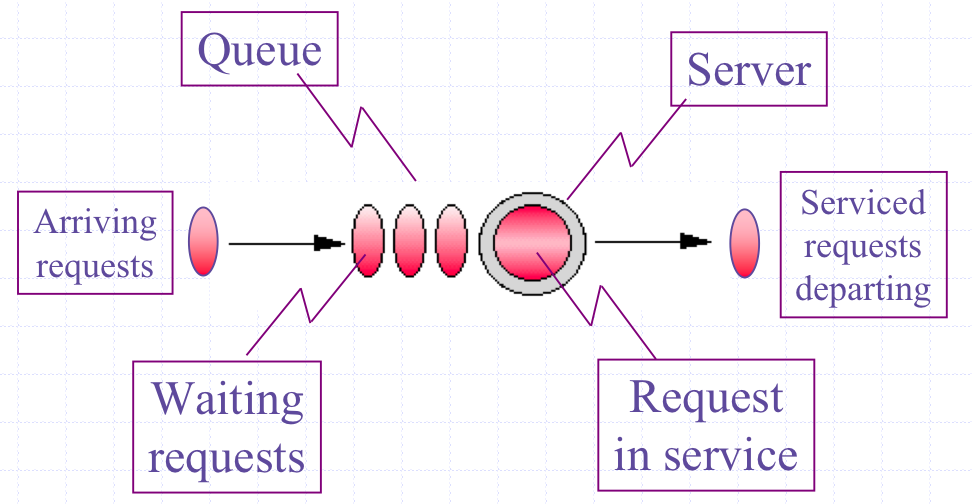
Figure 1: The components of an M/M/1 queue
The term "customer" is part of historical queueing parlence and might actually represent such things as:
- customers at a grocery checkout
- UNIX processes on the run-queue
- messages in a transaction monitor
- buffered packets at a router Accordingly, the "server" might represent
- the checkout stand
- a UNIX CPU
- transaction server
- a router CPU In queueing theory, this is known as an M/M/1 queue, meaning that both arrival and service periods are "Memoryless" or "M" (i.e., completely random in time) and there is only one server. Now, let's calculate the properties of the M/M/1 queue by hand. To do this, we need to recall the relevant mathematical relations for the M/M/1 queue.
4.1 M/M/1 Formulae
It is more convenient to think in terms of inputs and outputs. In other words, which parameters do we need to provide to the formulae versus those values we will calculate as the result of applying the formulae? We list them here:Inputs:
- The average arrival rate into the queue: λ.
- The average service time at the server: S. The Greek letters are part of the historical baggage in queueing theory and used in almost every textbook on the subject. There's no point trying to fight that now.
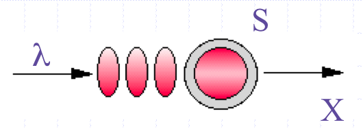
Figure 2: PDQ parameters for characterizing the M/M/1 queue in Figure 1
The throughtput, X, coming out of the server is the same as the arrival rate, λ coming into the queue because it is assumed to be in steady state. This point it discussed at length in _Analyzing Computer System Performance with Perl::PDQ_With these input parameters we can calculate all other performance quantities (outputs) of interest. Outputs:
- The average residence time a customer spends getting through the queueing system: R = S / (1 − λS)
- The average utilization of the server: ρ = λS
- The average queue length of the system: Q = λR
- The average waiting time a customer can expect to spend before getting service: W = R − S To apply these relationships, we need to choose some values for λ and S. We choose the following values so as to keep the arithmetic simple.Inputs:
- The average arrival rate: λ = 0.75 customers per second (or 3 customers every 4 seconds)
- The average service time: S = 1.0 second Then, the resulting queueing characteristics can be calculated using the above formulae.Outputs:
- R = 1.0 / (1 − 0.75 * 1.0) = 4.0 seconds (or 4 service periods)
- ρ = 0.75 or 75% (no units)
- Q = 0.75 * 4.0 = 3.0 customers
- W = 4.0 − 1.0 = 3.0 seconds For more realistic performance models we can combine a flow of "customers" between many different types pf queues; some like this one and others that are even more complex. Such calculations become extremely tedious and error-prone when you try to do them by hand. That's where PDQ comes in.
4.2 PDQ Model in Perl
In PDQ, the simple M/M/1 performance model described above would be coded in Perl as follows:
#!/usr/bin/perl
use pdq;
Globals
$arrivRate = 0.75; $servTime = 1.0;
Initialize PDQ and add a comment about the model
pdq::Init("Open Network with M/M/1"); pdq::SetComment("This is just a very simple example.");
Define the workload and circuit type
pdq::CreateOpen("Work", $arrivRate);
Define the queueing center
pdq::CreateNode("Server", pdq::CEN, pdq::CEN, pdq::CEN, pdq::FCFS);
Define service demand due to workload on the queueing center
pdq::SetDemand("Server", "Work", $servTime);
Change units labels to suit
pdq::SetWUnit("Cust"); pdq::SetTUnit("Secs");
Solve the model
Must use the Canonical method for an open network
pdq::Solve($pdq::CANON);
Generate a generic performance report
pdq::Report();
This might look like a lot of code for such a simple model, but realize that most of the code is for initialization and other set-up. When amortized over more realistic computer models, that becomes a much smaller fraction of the total code. Note also, that additional comment lines have been included to assist you in reading this particular model. In general, after some practice, you won't need those in every model.
4.3 PDQ Report
The corresponding standard PDQ report summarizes all the input parameters for the PDQ model, then outputs all the computed performance metrics.
PRETTY DAMN QUICK REPORT ========================================== *** on Mon Sep 7 17:19:18 2015 *** *** for Open Network with M/M/1 *** *** PDQ Version 6.2.0 Build 082015 *** ==========================================
COMMENT: This is just a very simple example.
========================================== ******** PDQ Model INPUTS ******** ==========================================
WORKLOAD Parameters:
Node Sched Resource Workload Class Demand ---- ----- -------- -------- ----- ------ 1 FCFS Server Work Open 1.0000
Queueing Circuit Totals Streams: 1 Nodes: 1
Arrivals per Secs Demand -------- -------- ------- Work 0.7500 1.0000
========================================== ******** PDQ Model OUTPUTS ******** ==========================================
Solution Method: CANON
******** SYSTEM Performance ********
Metric Value Unit ------ ----- ---- Workload: "Work" Number in system 3.0000 Cust Mean throughput 0.7500 Cust/Secs Response time 4.0000 Secs Stretch factor 4.0000
Bounds Analysis: Max throughput 1.0000 Cust/Secs Min response 1.0000 Secs
******** RESOURCE Performance ********
Metric Resource Work Value Unit ------ -------- ---- ----- ---- Capacity Server Work 1 Servers Throughput Server Work 0.7500 Cust/Secs In service Server Work 0.7500 Cust Utilization Server Work 75.0000 Percent Queue length Server Work 3.0000 Cust Waiting line Server Work 2.2500 Cust Waiting time Server Work 3.0000 Secs Residence time Server Work 4.0000 Secs
We see that the PDQ results are in complete agreement with those previously calculated by hand using the M/M/1 formulae in Section 4.1. A more detailed discussion is presented in Chapter 8 ofAnalyzing Computer System Performance with Perl::PDQ. Copyright © 2005—2025 Performance Dynamics Company. All Rights Reserved.
Updated on Wed Jul 13 06:43:56 PDT 2022