ggcorrplot: Visualization of a correlation matrix using ggplot2 - Easy Guides - Wiki (original) (raw)

1. Home
2. Easy Guides
3. R software
4. Data Visualization
5. ggplot2 - Essentials
6. ggcorrplot: Visualization of a correlation matrix using ggplot2

• ggcorrplot main features
• Installation and loading
• Getting started
  • Compute a correlation matrix
  • Correlation matrix visualization

The easiest way to visualize a correlation matrix in R is to use the package corrplot.

In our previous article we also provided a quick-start guide for visualizing a correlation matrix using ggplot2.

Another solution is to use the function ggcorr() in ggally package. However, the ggally package doesn’t provide any option for reordering the correlation matrix or for displaying the significance level.

In this article, we’ll describe the R package ggcorrplot for displaying easily a correlation matrix using ‘ggplot2’.

ggcorrplot main features

It provides a solution for reordering the correlation matrix and displays the significance level on the correlogram. It includes also a function for computing a matrix of correlation p-values. It’s inspired from the package corrplot.

Installation and loading

ggcorrplot can be installed from CRAN as follow:

install.packages("ggcorrplot")

Or, install the latest version from GitHub:

# Install
if(!require(devtools)) install.packages("devtools")
devtools::install_github("kassambara/ggcorrplot")

Loading:

library(ggcorrplot)

Getting started

Compute a correlation matrix

The mtcars data set will be used in the following R code. The function cor_pmat() [in ggcorrplot] computes a matrix of correlation p-values.

# Compute a correlation matrix
data(mtcars)
corr <- round(cor(mtcars), 1)
head(corr[, 1:6])

##       mpg  cyl disp   hp drat   wt
## mpg   1.0 -0.9 -0.8 -0.8  0.7 -0.9
## cyl  -0.9  1.0  0.9  0.8 -0.7  0.8
## disp -0.8  0.9  1.0  0.8 -0.7  0.9
## hp   -0.8  0.8  0.8  1.0 -0.4  0.7
## drat  0.7 -0.7 -0.7 -0.4  1.0 -0.7
## wt   -0.9  0.8  0.9  0.7 -0.7  1.0

# Compute a matrix of correlation p-values
p.mat <- cor_pmat(mtcars)
head(p.mat[, 1:4])

##               mpg          cyl         disp           hp
## mpg  0.000000e+00 6.112687e-10 9.380327e-10 1.787835e-07
## cyl  6.112687e-10 0.000000e+00 1.803002e-12 3.477861e-09
## disp 9.380327e-10 1.803002e-12 0.000000e+00 7.142679e-08
## hp   1.787835e-07 3.477861e-09 7.142679e-08 0.000000e+00
## drat 1.776240e-05 8.244636e-06 5.282022e-06 9.988772e-03
## wt   1.293959e-10 1.217567e-07 1.222311e-11 4.145827e-05

Correlation matrix visualization

# Visualize the correlation matrix
# --------------------------------
# method = "square" (default)
ggcorrplot(corr)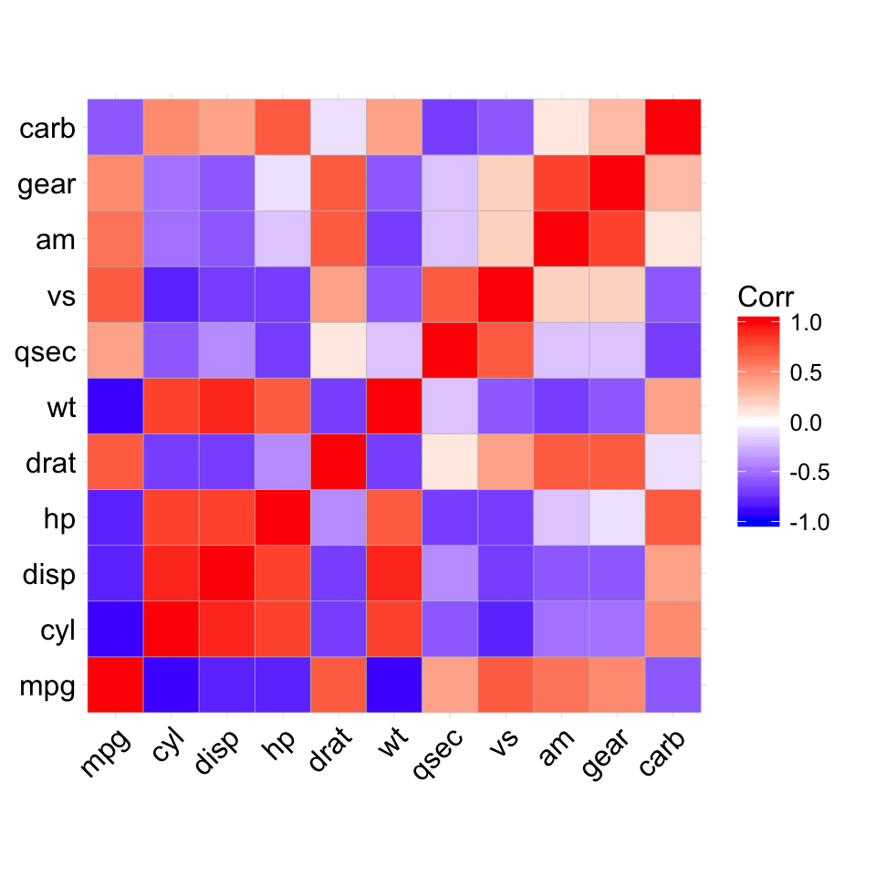

# method = "circle"
ggcorrplot(corr, method = "circle")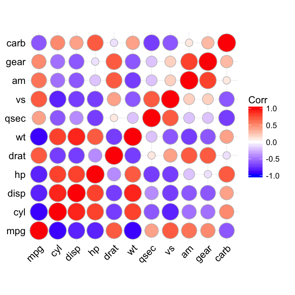

# Reordering the correlation matrix
# --------------------------------
# using hierarchical clustering
ggcorrplot(corr, hc.order = TRUE, outline.col = "white")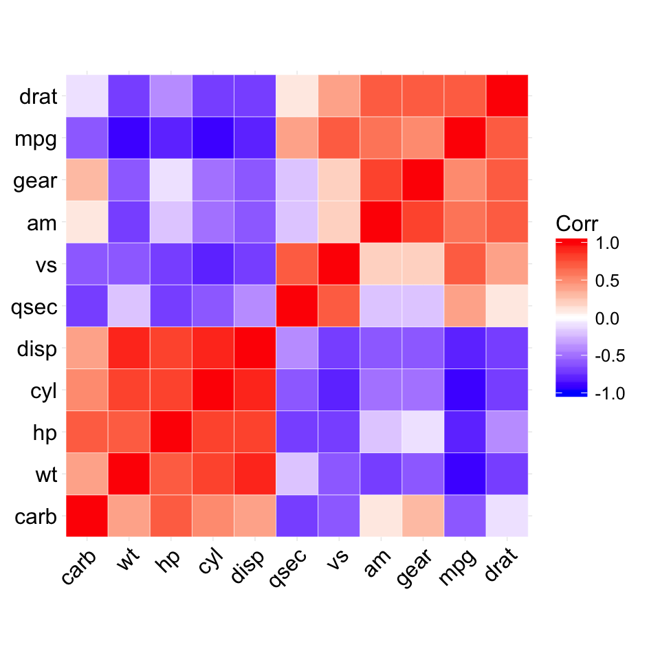

# Types of correlogram layout
# --------------------------------
# Get the lower triangle
ggcorrplot(corr, hc.order = TRUE, type = "lower",
     outline.col = "white")

# Get the upeper triangle
ggcorrplot(corr, hc.order = TRUE, type = "upper",
     outline.col = "white")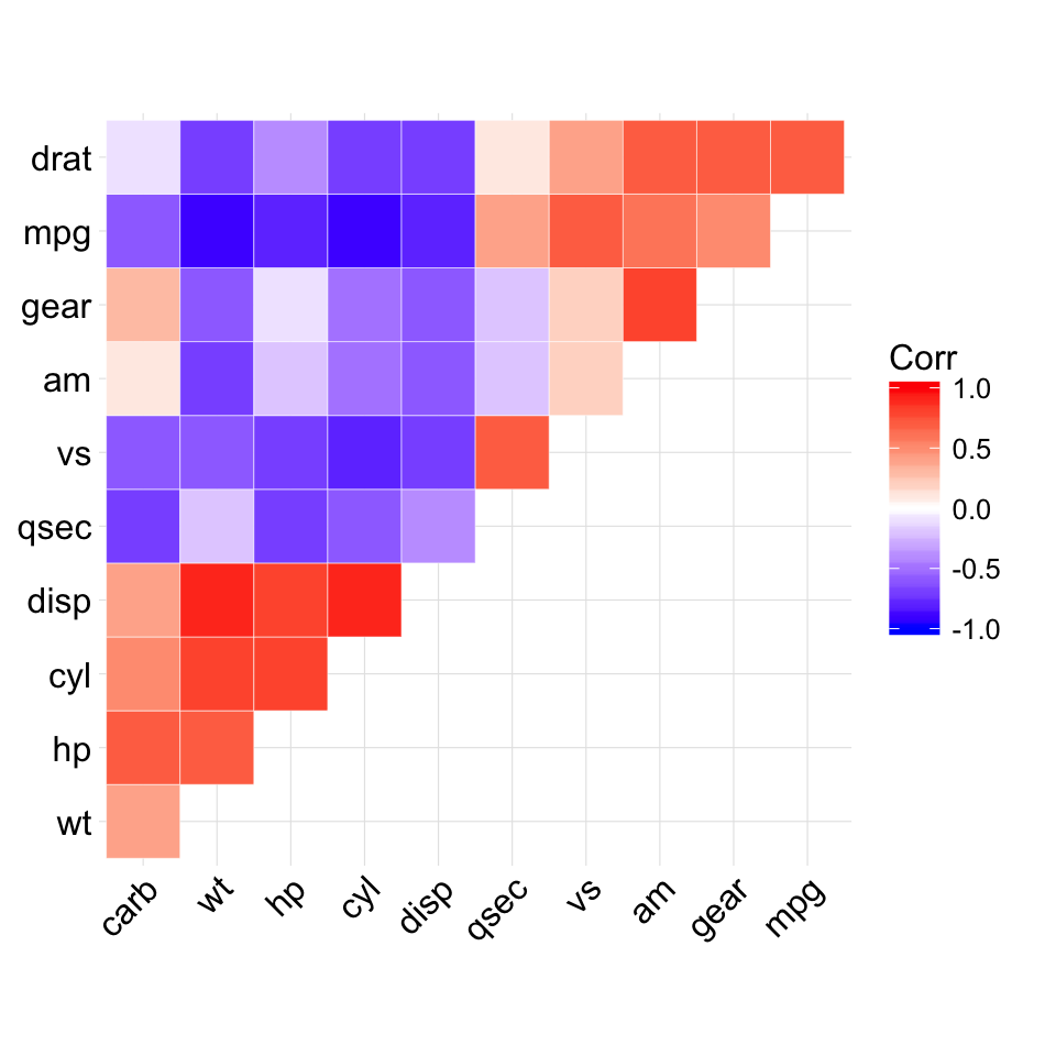

# Change colors and theme
# --------------------------------
# Argument colors
ggcorrplot(corr, hc.order = TRUE, type = "lower",
   outline.col = "white",
   ggtheme = ggplot2::theme_gray,
   colors = c("#6D9EC1", "white", "#E46726"))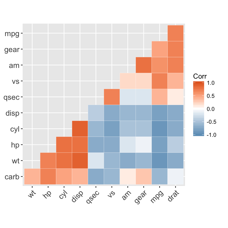

# Add correlation coefficients
# --------------------------------
# argument lab = TRUE
ggcorrplot(corr, hc.order = TRUE, type = "lower",
   lab = TRUE)

# Add correlation significance level
# --------------------------------
# Argument p.mat
# Barring the no significant coefficient
ggcorrplot(corr, hc.order = TRUE,
    type = "lower", p.mat = p.mat)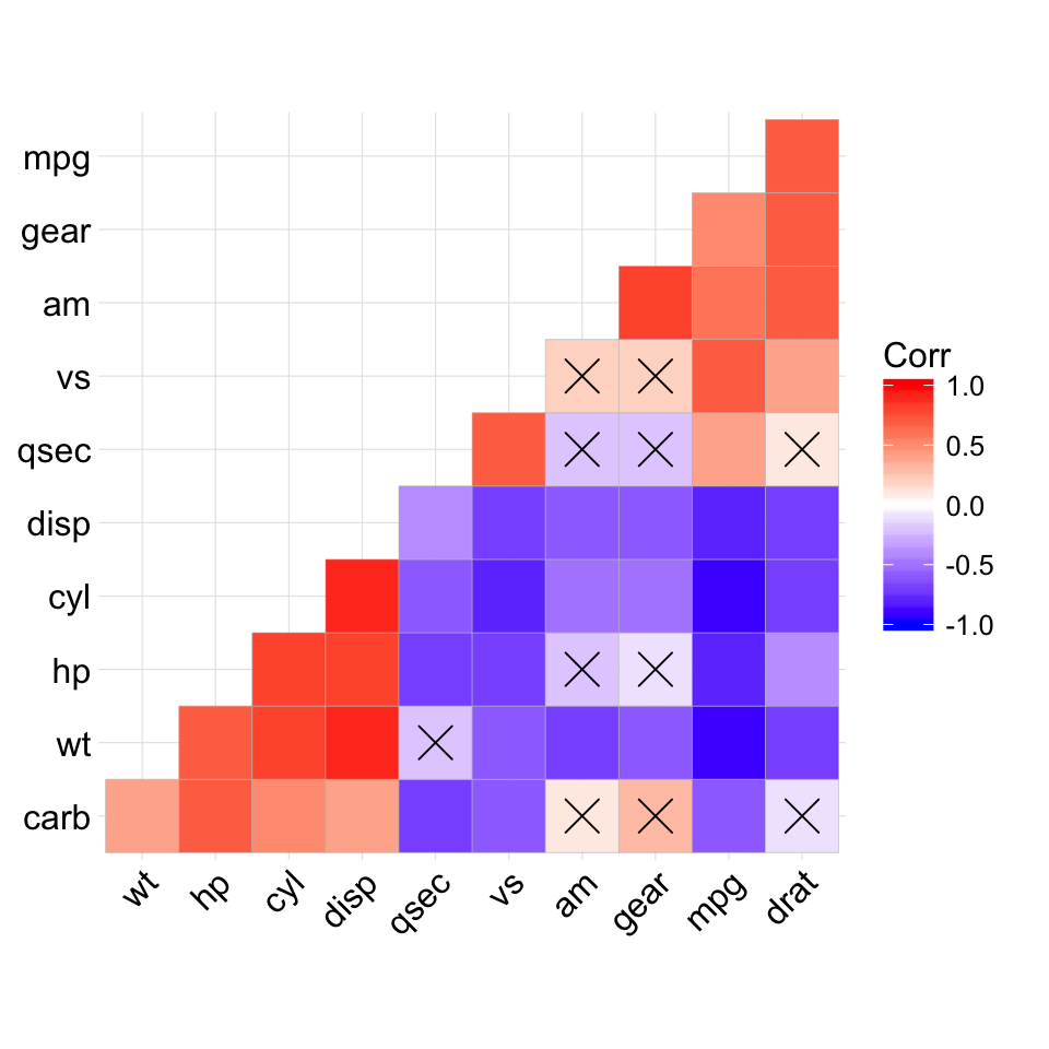

# Leave blank on no significant coefficient
ggcorrplot(corr, p.mat = p.mat, hc.order = TRUE,
    type = "lower", insig = "blank")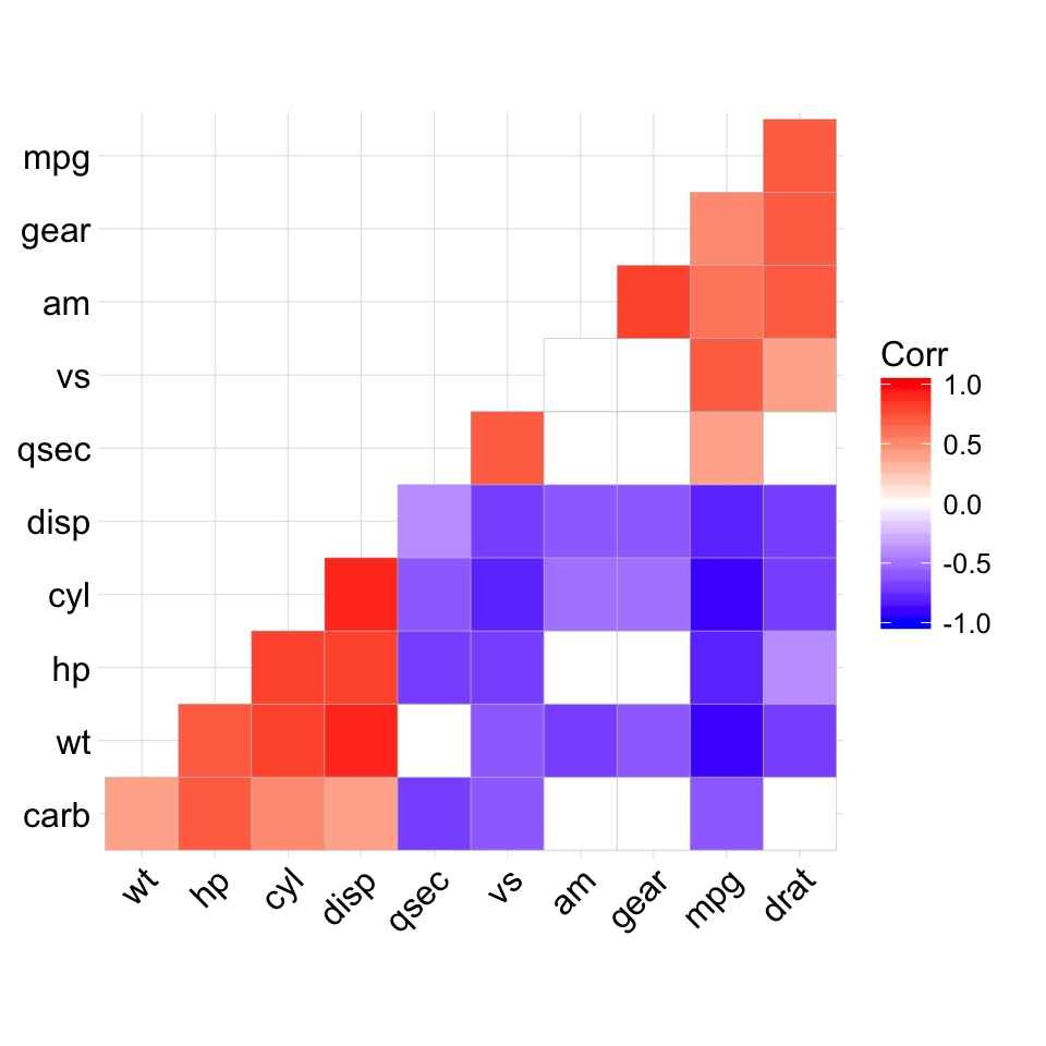

Enjoyed this article? I’d be very grateful if you’d help it spread by emailing it to a friend, or sharing it on Twitter, Facebook or Linked In.

Show me some love with the like buttons below... Thank you and please don't forget to share and comment below!!

Avez vous aimé cet article? Je vous serais très reconnaissant si vous aidiez à sa diffusion en l'envoyant par courriel à un ami ou en le partageant sur Twitter, Facebook ou Linked In.

Montrez-moi un peu d'amour avec les like ci-dessous ... Merci et n'oubliez pas, s'il vous plaît, de partager et de commenter ci-dessous!

Recommended for You!

Get involved :
Click to follow us on Facebook :
Comment this article by clicking on "Discussion" button (top-right position of this page)