ev — SciPy v1.15.3 Manual (original) (raw)

scipy.interpolate.SmoothSphereBivariateSpline.

SmoothSphereBivariateSpline.ev(theta, phi, dtheta=0, dphi=0)[source]#

Evaluate the spline at points

Returns the interpolated value at (theta[i], phi[i]), i=0,...,len(theta)-1.

Parameters:

theta, phiarray_like

Input coordinates. Standard Numpy broadcasting is obeyed. The ordering of axes is consistent with np.meshgrid(…, indexing=”ij”) and inconsistent with the default ordering np.meshgrid(…, indexing=”xy”).

dthetaint, optional

Order of theta-derivative

Added in version 0.14.0.

dphiint, optional

Order of phi-derivative

Added in version 0.14.0.

Examples

Suppose that we want to use splines to interpolate a bivariate function on a sphere. The value of the function is known on a grid of longitudes and colatitudes.

import numpy as np from scipy.interpolate import RectSphereBivariateSpline def f(theta, phi): ... return np.sin(theta) * np.cos(phi)

We evaluate the function on the grid. Note that the default indexing=”xy” of meshgrid would result in an unexpected (transposed) result after interpolation.

thetaarr = np.linspace(0, np.pi, 22)[1:-1] phiarr = np.linspace(0, 2 * np.pi, 21)[:-1] thetagrid, phigrid = np.meshgrid(thetaarr, phiarr, indexing="ij") zdata = f(thetagrid, phigrid)

We next set up the interpolator and use it to evaluate the function at points not on the original grid.

rsbs = RectSphereBivariateSpline(thetaarr, phiarr, zdata) thetainterp = np.linspace(thetaarr[0], thetaarr[-1], 200) phiinterp = np.linspace(phiarr[0], phiarr[-1], 200) zinterp = rsbs.ev(thetainterp, phiinterp)

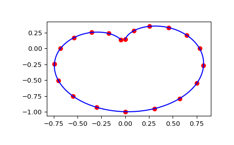
Finally we plot the original data for a diagonal slice through the initial grid, and the spline approximation along the same slice.

import matplotlib.pyplot as plt fig = plt.figure() ax1 = fig.add_subplot(1, 1, 1) ax1.plot(np.sin(thetaarr) * np.sin(phiarr), np.diag(zdata), "or") ax1.plot(np.sin(thetainterp) * np.sin(phiinterp), zinterp, "-b") plt.show()