Computational tools — pandas 0.16.2 documentation (original) (raw)

Statistical functions¶

Percent Change¶

Series, DataFrame, and Panel all have a method pct_change to compute the percent change over a given number of periods (using fill_method to fill NA/null values before computing the percent change).

In [1]: ser = pd.Series(np.random.randn(8))

In [2]: ser.pct_change() Out[2]: 0 NaN 1 -1.602976 2 4.334938 3 -0.247456 4 -2.067345 5 -1.142903 6 -1.688214 7 -9.759729 dtype: float64

In [3]: df = pd.DataFrame(np.random.randn(10, 4))

In [4]: df.pct_change(periods=3) Out[4]: 0 1 2 3 0 NaN NaN NaN NaN 1 NaN NaN NaN NaN 2 NaN NaN NaN NaN 3 -0.218320 -1.054001 1.987147 -0.510183 4 -0.439121 -1.816454 0.649715 -4.822809 5 -0.127833 -3.042065 -5.866604 -1.776977 6 -2.596833 -1.959538 -2.111697 -3.798900 7 -0.117826 -2.169058 0.036094 -0.067696 8 2.492606 -1.357320 -1.205802 -1.558697 9 -1.012977 2.324558 -1.003744 -0.371806

Covariance¶

The Series object has a method cov to compute covariance between series (excluding NA/null values).

In [5]: s1 = pd.Series(np.random.randn(1000))

In [6]: s2 = pd.Series(np.random.randn(1000))

In [7]: s1.cov(s2) Out[7]: 0.00068010881743109993

Analogously, DataFrame has a method cov to compute pairwise covariances among the series in the DataFrame, also excluding NA/null values.

Note

Assuming the missing data are missing at random this results in an estimate for the covariance matrix which is unbiased. However, for many applications this estimate may not be acceptable because the estimated covariance matrix is not guaranteed to be positive semi-definite. This could lead to estimated correlations having absolute values which are greater than one, and/or a non-invertible covariance matrix. See Estimation of covariance matricesfor more details.

In [8]: frame = pd.DataFrame(np.random.randn(1000, 5), columns=['a', 'b', 'c', 'd', 'e'])

In [9]: frame.cov() Out[9]: a b c d e a 1.000882 -0.003177 -0.002698 -0.006889 0.031912 b -0.003177 1.024721 0.000191 0.009212 0.000857 c -0.002698 0.000191 0.950735 -0.031743 -0.005087 d -0.006889 0.009212 -0.031743 1.002983 -0.047952 e 0.031912 0.000857 -0.005087 -0.047952 1.042487

DataFrame.cov also supports an optional min_periods keyword that specifies the required minimum number of observations for each column pair in order to have a valid result.

In [10]: frame = pd.DataFrame(np.random.randn(20, 3), columns=['a', 'b', 'c'])

In [11]: frame.ix[:5, 'a'] = np.nan

In [12]: frame.ix[5:10, 'b'] = np.nan

In [13]: frame.cov() Out[13]: a b c a 1.210090 -0.430629 0.018002 b -0.430629 1.240960 0.347188 c 0.018002 0.347188 1.301149

In [14]: frame.cov(min_periods=12) Out[14]: a b c a 1.210090 NaN 0.018002 b NaN 1.240960 0.347188 c 0.018002 0.347188 1.301149

Correlation¶

Several methods for computing correlations are provided:

Method name	Description
pearson (default)	Standard correlation coefficient
kendall	Kendall Tau correlation coefficient
spearman	Spearman rank correlation coefficient

All of these are currently computed using pairwise complete observations.

Note

Please see the caveats associated with this method of calculating correlation matrices in thecovariance section.

In [15]: frame = pd.DataFrame(np.random.randn(1000, 5), columns=['a', 'b', 'c', 'd', 'e'])

In [16]: frame.ix[::2] = np.nan

Series with Series

In [17]: frame['a'].corr(frame['b']) Out[17]: 0.013479040400098794

In [18]: frame['a'].corr(frame['b'], method='spearman') Out[18]: -0.0072898851595406388

Pairwise correlation of DataFrame columns

In [19]: frame.corr() Out[19]: a b c d e a 1.000000 0.013479 -0.049269 -0.042239 -0.028525 b 0.013479 1.000000 -0.020433 -0.011139 0.005654 c -0.049269 -0.020433 1.000000 0.018587 -0.054269 d -0.042239 -0.011139 0.018587 1.000000 -0.017060 e -0.028525 0.005654 -0.054269 -0.017060 1.000000

Note that non-numeric columns will be automatically excluded from the correlation calculation.

Like cov, corr also supports the optional min_periods keyword:

In [20]: frame = pd.DataFrame(np.random.randn(20, 3), columns=['a', 'b', 'c'])

In [21]: frame.ix[:5, 'a'] = np.nan

In [22]: frame.ix[5:10, 'b'] = np.nan

In [23]: frame.corr() Out[23]: a b c a 1.000000 -0.076520 0.160092 b -0.076520 1.000000 0.135967 c 0.160092 0.135967 1.000000

In [24]: frame.corr(min_periods=12) Out[24]: a b c a 1.000000 NaN 0.160092 b NaN 1.000000 0.135967 c 0.160092 0.135967 1.000000

A related method corrwith is implemented on DataFrame to compute the correlation between like-labeled Series contained in different DataFrame objects.

In [25]: index = ['a', 'b', 'c', 'd', 'e']

In [26]: columns = ['one', 'two', 'three', 'four']

In [27]: df1 = pd.DataFrame(np.random.randn(5, 4), index=index, columns=columns)

In [28]: df2 = pd.DataFrame(np.random.randn(4, 4), index=index[:4], columns=columns)

In [29]: df1.corrwith(df2) Out[29]: one -0.125501 two -0.493244 three 0.344056 four 0.004183 dtype: float64

In [30]: df2.corrwith(df1, axis=1) Out[30]: a -0.675817 b 0.458296 c 0.190809 d -0.186275 e NaN dtype: float64

Data ranking¶

The rank method produces a data ranking with ties being assigned the mean of the ranks (by default) for the group:

In [31]: s = pd.Series(np.random.np.random.randn(5), index=list('abcde'))

In [32]: s['d'] = s['b'] # so there's a tie

In [33]: s.rank() Out[33]: a 5.0 b 2.5 c 1.0 d 2.5 e 4.0 dtype: float64

rank is also a DataFrame method and can rank either the rows (axis=0) or the columns (axis=1). NaN values are excluded from the ranking.

In [34]: df = pd.DataFrame(np.random.np.random.randn(10, 6))

In [35]: df[4] = df[2][:5] # some ties

In [36]: df Out[36]: 0 1 2 3 4 5 0 -0.904948 -1.163537 -1.457187 0.135463 -1.457187 0.294650 1 -0.976288 -0.244652 -0.748406 -0.999601 -0.748406 -0.800809 2 0.401965 1.460840 1.256057 1.308127 1.256057 0.876004 3 0.205954 0.369552 -0.669304 0.038378 -0.669304 1.140296 4 -0.477586 -0.730705 -1.129149 -0.601463 -1.129149 -0.211196 5 -1.092970 -0.689246 0.908114 0.204848 NaN 0.463347 6 0.376892 0.959292 0.095572 -0.593740 NaN -0.069180 7 -1.002601 1.957794 -0.120708 0.094214 NaN -1.467422 8 -0.547231 0.664402 -0.519424 -0.073254 NaN -1.263544 9 -0.250277 -0.237428 -1.056443 0.419477 NaN 1.375064

In [37]: df.rank(1) Out[37]: 0 1 2 3 4 5 0 4 3 1.5 5 1.5 6 1 2 6 4.5 1 4.5 3 2 1 6 3.5 5 3.5 2 3 4 5 1.5 3 1.5 6 4 5 3 1.5 4 1.5 6 5 1 2 5.0 3 NaN 4 6 4 5 3.0 1 NaN 2 7 2 5 3.0 4 NaN 1 8 2 5 3.0 4 NaN 1 9 2 3 1.0 4 NaN 5

rank optionally takes a parameter ascending which by default is true; when false, data is reverse-ranked, with larger values assigned a smaller rank.

rank supports different tie-breaking methods, specified with the methodparameter:

average : average rank of tied group

min : lowest rank in the group

max : highest rank in the group

first : ranks assigned in the order they appear in the array

Moving (rolling) statistics / moments¶

For working with time series data, a number of functions are provided for computing common moving or rolling statistics. Among these are count, sum, mean, median, correlation, variance, covariance, standard deviation, skewness, and kurtosis. All of these methods are in the pandas namespace, but otherwise they can be found in pandas.stats.moments.

Function	Description
rolling_count	Number of non-null observations
rolling_sum	Sum of values
rolling_mean	Mean of values
rolling_median	Arithmetic median of values
rolling_min	Minimum
rolling_max	Maximum
rolling_std	Unbiased standard deviation
rolling_var	Unbiased variance
rolling_skew	Unbiased skewness (3rd moment)
rolling_kurt	Unbiased kurtosis (4th moment)
rolling_quantile	Sample quantile (value at %)
rolling_apply	Generic apply
rolling_cov	Unbiased covariance (binary)
rolling_corr	Correlation (binary)
rolling_window	Moving window function

Generally these methods all have the same interface. The binary operators (e.g. rolling_corr) take two Series or DataFrames. Otherwise, they all accept the following arguments:

window: size of moving window

min_periods: threshold of non-null data points to require (otherwise result is NA)

freq: optionally specify a frequency stringor DateOffset to pre-conform the data to. Note that prior to pandas v0.8.0, a keyword argument time_rule was used instead of freq that referred to the legacy time rule constants

how: optionally specify method for down or re-sampling. Default is is min for rolling_min, max for rolling_max, median forrolling_median, and mean for all other rolling functions. SeeDataFrame.resample()‘s how argument for more information.

These functions can be applied to ndarrays or Series objects:

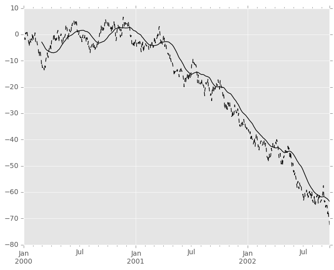
In [38]: ts = pd.Series(np.random.randn(1000), index=pd.date_range('1/1/2000', periods=1000))

In [39]: ts = ts.cumsum()

In [40]: ts.plot(style='k--') Out[40]: <matplotlib.axes._subplots.AxesSubplot at 0xa95eda2c>

In [41]: pd.rolling_mean(ts, 60).plot(style='k') Out[41]: <matplotlib.axes._subplots.AxesSubplot at 0xa95eda2c>

_images/rolling_mean_ex.png

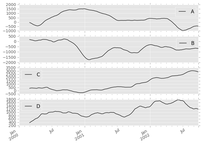
They can also be applied to DataFrame objects. This is really just syntactic sugar for applying the moving window operator to all of the DataFrame’s columns:

In [42]: df = pd.DataFrame(np.random.randn(1000, 4), index=ts.index, ....: columns=['A', 'B', 'C', 'D']) ....:

In [43]: df = df.cumsum()

In [44]: pd.rolling_sum(df, 60).plot(subplots=True) Out[44]: array([<matplotlib.axes._subplots.AxesSubplot object at 0xaa23020c>, <matplotlib.axes._subplots.AxesSubplot object at 0xaa0c410c>, <matplotlib.axes._subplots.AxesSubplot object at 0xaa0a592c>, <matplotlib.axes._subplots.AxesSubplot object at 0xaa159e4c>], dtype=object)

_images/rolling_mean_frame.png

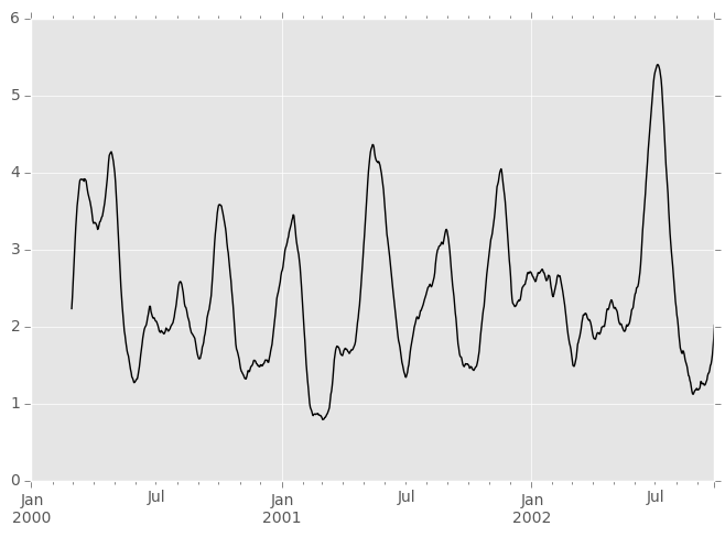
The rolling_apply function takes an extra func argument and performs generic rolling computations. The func argument should be a single function that produces a single value from an ndarray input. Suppose we wanted to compute the mean absolute deviation on a rolling basis:

In [45]: mad = lambda x: np.fabs(x - x.mean()).mean()

In [46]: pd.rolling_apply(ts, 60, mad).plot(style='k') Out[46]: <matplotlib.axes._subplots.AxesSubplot at 0xa9b4b84c>

_images/rolling_apply_ex.png

The rolling_window function performs a generic rolling window computation on the input data. The weights used in the window are specified by the win_typekeyword. The list of recognized types are:

boxcar

triang

blackman

hamming

bartlett

parzen

bohman

blackmanharris

nuttall

barthann

kaiser (needs beta)

gaussian (needs std)

general_gaussian (needs power, width)

slepian (needs width).

In [47]: ser = pd.Series(np.random.randn(10), index=pd.date_range('1/1/2000', periods=10))

In [48]: pd.rolling_window(ser, 5, 'triang') Out[48]: 2000-01-01 NaN 2000-01-02 NaN 2000-01-03 NaN 2000-01-04 NaN 2000-01-05 -1.037870 2000-01-06 -0.767705 2000-01-07 -0.383197 2000-01-08 -0.395513 2000-01-09 -0.558440 2000-01-10 -0.672416 Freq: D, dtype: float64

Note that the boxcar window is equivalent to rolling_mean.

In [49]: pd.rolling_window(ser, 5, 'boxcar') Out[49]: 2000-01-01 NaN 2000-01-02 NaN 2000-01-03 NaN 2000-01-04 NaN 2000-01-05 -0.841164 2000-01-06 -0.779948 2000-01-07 -0.565487 2000-01-08 -0.502815 2000-01-09 -0.553755 2000-01-10 -0.472211 Freq: D, dtype: float64

In [50]: pd.rolling_mean(ser, 5) Out[50]: 2000-01-01 NaN 2000-01-02 NaN 2000-01-03 NaN 2000-01-04 NaN 2000-01-05 -0.841164 2000-01-06 -0.779948 2000-01-07 -0.565487 2000-01-08 -0.502815 2000-01-09 -0.553755 2000-01-10 -0.472211 Freq: D, dtype: float64

For some windowing functions, additional parameters must be specified:

In [51]: pd.rolling_window(ser, 5, 'gaussian', std=0.1) Out[51]: 2000-01-01 NaN 2000-01-02 NaN 2000-01-03 NaN 2000-01-04 NaN 2000-01-05 -1.309989 2000-01-06 -1.153000 2000-01-07 0.606382 2000-01-08 -0.681101 2000-01-09 -0.289724 2000-01-10 -0.996632 Freq: D, dtype: float64

By default the labels are set to the right edge of the window, but acenter keyword is available so the labels can be set at the center. This keyword is available in other rolling functions as well.

In [52]: pd.rolling_window(ser, 5, 'boxcar') Out[52]: 2000-01-01 NaN 2000-01-02 NaN 2000-01-03 NaN 2000-01-04 NaN 2000-01-05 -0.841164 2000-01-06 -0.779948 2000-01-07 -0.565487 2000-01-08 -0.502815 2000-01-09 -0.553755 2000-01-10 -0.472211 Freq: D, dtype: float64

In [53]: pd.rolling_window(ser, 5, 'boxcar', center=True) Out[53]: 2000-01-01 NaN 2000-01-02 NaN 2000-01-03 -0.841164 2000-01-04 -0.779948 2000-01-05 -0.565487 2000-01-06 -0.502815 2000-01-07 -0.553755 2000-01-08 -0.472211 2000-01-09 NaN 2000-01-10 NaN Freq: D, dtype: float64

In [54]: pd.rolling_mean(ser, 5, center=True) Out[54]: 2000-01-01 NaN 2000-01-02 NaN 2000-01-03 -0.841164 2000-01-04 -0.779948 2000-01-05 -0.565487 2000-01-06 -0.502815 2000-01-07 -0.553755 2000-01-08 -0.472211 2000-01-09 NaN 2000-01-10 NaN Freq: D, dtype: float64

Note

In rolling sum mode (mean=False) there is no normalization done to the weights. Passing custom weights of [1, 1, 1] will yield a different result than passing weights of [2, 2, 2], for example. When passing awin_type instead of explicitly specifying the weights, the weights are already normalized so that the largest weight is 1.

In contrast, the nature of the rolling mean calculation (mean=True)is such that the weights are normalized with respect to each other. Weights of [1, 1, 1] and [2, 2, 2] yield the same result.

Binary rolling moments¶

rolling_cov and rolling_corr can compute moving window statistics about two Series or any combination of DataFrame/Series orDataFrame/DataFrame. Here is the behavior in each case:

two Series: compute the statistic for the pairing.
DataFrame/Series: compute the statistics for each column of the DataFrame with the passed Series, thus returning a DataFrame.
DataFrame/DataFrame: by default compute the statistic for matching column names, returning a DataFrame. If the keyword argument pairwise=True is passed then computes the statistic for each pair of columns, returning aPanel whose items are the dates in question (see the next section).

For example:

In [55]: df2 = df[:20]

In [56]: pd.rolling_corr(df2, df2['B'], window=5) Out[56]: A B C D 2000-01-01 NaN NaN NaN NaN 2000-01-02 NaN NaN NaN NaN 2000-01-03 NaN NaN NaN NaN 2000-01-04 NaN NaN NaN NaN 2000-01-05 -0.262853 1 0.334449 0.193380 2000-01-06 -0.083745 1 -0.521587 -0.556126 2000-01-07 -0.292940 1 -0.658532 -0.458128 ... ... .. ... ... 2000-01-14 0.519499 1 -0.687277 0.192822 2000-01-15 0.048982 1 0.167669 -0.061463 2000-01-16 0.217190 1 0.167564 -0.326034 2000-01-17 0.641180 1 -0.164780 -0.111487 2000-01-18 0.130422 1 0.322833 0.632383 2000-01-19 0.317278 1 0.384528 0.813656 2000-01-20 0.293598 1 0.159538 0.742381

[20 rows x 4 columns]

Computing rolling pairwise covariances and correlations¶

In financial data analysis and other fields it’s common to compute covariance and correlation matrices for a collection of time series. Often one is also interested in moving-window covariance and correlation matrices. This can be done by passing the pairwise keyword argument, which in the case ofDataFrame inputs will yield a Panel whose items are the dates in question. In the case of a single DataFrame argument the pairwise argument can even be omitted:

Note

Missing values are ignored and each entry is computed using the pairwise complete observations. Please see the covariance section for caveats associated with this method of calculating covariance and correlation matrices.

In [57]: covs = pd.rolling_cov(df[['B','C','D']], df[['A','B','C']], 50, pairwise=True)

In [58]: covs[df.index[-50]] Out[58]: A B C B 2.667506 1.671711 1.938634 C 8.513843 1.938634 10.556436 D -7.714737 -1.434529 -7.082653

In [59]: correls = pd.rolling_corr(df, 50)

In [60]: correls[df.index[-50]] Out[60]: A B C D A 1.000000 0.604221 0.767429 -0.776170 B 0.604221 1.000000 0.461484 -0.381148 C 0.767429 0.461484 1.000000 -0.748863 D -0.776170 -0.381148 -0.748863 1.000000

Note

Prior to version 0.14 this was available through rolling_corr_pairwisewhich is now simply syntactic sugar for calling rolling_corr(..., pairwise=True) and deprecated. This is likely to be removed in a future release.

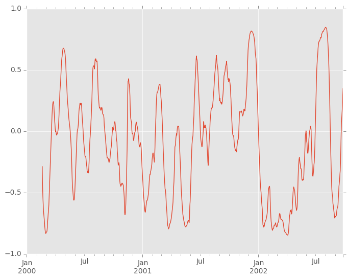
You can efficiently retrieve the time series of correlations between two columns using ix indexing:

In [61]: correls.ix[:, 'A', 'C'].plot() Out[61]: <matplotlib.axes._subplots.AxesSubplot at 0xa63e68ac>

_images/rolling_corr_pairwise_ex.png

Expanding window moment functions¶

A common alternative to rolling statistics is to use an expanding window, which yields the value of the statistic with all the data available up to that point in time. As these calculations are a special case of rolling statistics, they are implemented in pandas such that the following two calls are equivalent:

In [62]: pd.rolling_mean(df, window=len(df), min_periods=1)[:5] Out[62]: A B C D 2000-01-01 -1.388345 3.317290 0.344542 -0.036968 2000-01-02 -1.123132 3.622300 1.675867 0.595300 2000-01-03 -0.628502 3.626503 2.455240 1.060158 2000-01-04 -0.768740 3.888917 2.451354 1.281874 2000-01-05 -0.824034 4.108035 2.556112 1.140723

In [63]: pd.expanding_mean(df)[:5] Out[63]: A B C D 2000-01-01 -1.388345 3.317290 0.344542 -0.036968 2000-01-02 -1.123132 3.622300 1.675867 0.595300 2000-01-03 -0.628502 3.626503 2.455240 1.060158 2000-01-04 -0.768740 3.888917 2.451354 1.281874 2000-01-05 -0.824034 4.108035 2.556112 1.140723

Like the rolling_ functions, the following methods are included in thepandas namespace or can be located in pandas.stats.moments.

Function	Description
expanding_count	Number of non-null observations
expanding_sum	Sum of values
expanding_mean	Mean of values
expanding_median	Arithmetic median of values
expanding_min	Minimum
expanding_max	Maximum
expanding_std	Unbiased standard deviation
expanding_var	Unbiased variance
expanding_skew	Unbiased skewness (3rd moment)
expanding_kurt	Unbiased kurtosis (4th moment)
expanding_quantile	Sample quantile (value at %)
expanding_apply	Generic apply
expanding_cov	Unbiased covariance (binary)
expanding_corr	Correlation (binary)

Aside from not having a window parameter, these functions have the same interfaces as their rolling_ counterpart. Like above, the parameters they all accept are:

min_periods: threshold of non-null data points to require. Defaults to minimum needed to compute statistic. No NaNs will be output oncemin_periods non-null data points have been seen.

freq: optionally specify a frequency stringor DateOffset to pre-conform the data to. Note that prior to pandas v0.8.0, a keyword argument time_rule was used instead of freq that referred to the legacy time rule constants

Note

The output of the rolling_ and expanding_ functions do not return aNaN if there are at least min_periods non-null values in the current window. This differs from cumsum, cumprod, cummax, andcummin, which return NaN in the output wherever a NaN is encountered in the input.

An expanding window statistic will be more stable (and less responsive) than its rolling window counterpart as the increasing window size decreases the relative impact of an individual data point. As an example, here is theexpanding_mean output for the previous time series dataset:

In [64]: ts.plot(style='k--') Out[64]: <matplotlib.axes._subplots.AxesSubplot at 0xa9ba130c>

In [65]: pd.expanding_mean(ts).plot(style='k') Out[65]: <matplotlib.axes._subplots.AxesSubplot at 0xa9ba130c>

_images/expanding_mean_frame.png

Exponentially weighted moment functions¶

A related set of functions are exponentially weighted versions of several of the above statistics. A number of expanding EW (exponentially weighted) functions are provided:

Function	Description
ewma	EW moving average
ewmvar	EW moving variance
ewmstd	EW moving standard deviation
ewmcorr	EW moving correlation
ewmcov	EW moving covariance

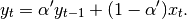
In general, a weighted moving average is calculated as

$y_t = \frac{\sum_{i=0}^t w_i x_{t-i}}{\sum_{i=0}^t w_i},$

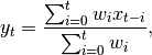
where $x_t$ is the input at $y_t$ is the result.

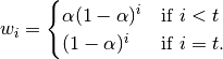
The EW functions support two variants of exponential weights: The default, adjust=True, uses the weights 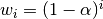$w_i = (1 - \alpha)^i$ . When adjust=False is specified, moving averages are calculated as

$y_0 &= x_0 \\ y_t &= (1 - \alpha) y_{t-1} + \alpha x_t,$

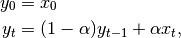
which is equivalent to using weights

$w_i = \begin{cases} \alpha (1 - \alpha)^i & \text{if } i < t \\ (1 - \alpha)^i & \text{if } i = t. \end{cases}$

Note

These equations are sometimes written in terms of $\alpha' = 1 - \alpha$ , e.g.

$y_t = \alpha' y_{t-1} + (1 - \alpha') x_t.$

One must have $0 < \alpha \leq 1$ , but rather than pass $\alpha$ directly, it’s easier to think about either the span, center of mass (com) or halflife of an EW moment:

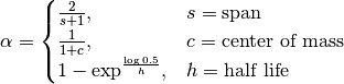
$\alpha = \begin{cases} \frac{2}{s + 1}, & s = \text{span}\\ \frac{1}{1 + c}, & c = \text{center of mass}\\ 1 - \exp^{\frac{\log 0.5}{h}}, & h = \text{half life} \end{cases}$

One must specify precisely one of the three to the EW functions. Spancorresponds to what is commonly called a “20-day EW moving average” for example. Center of mass has a more physical interpretation. For example,span = 20 corresponds to com = 9.5. Halflife is the period of time for the exponential weight to reduce to one half.

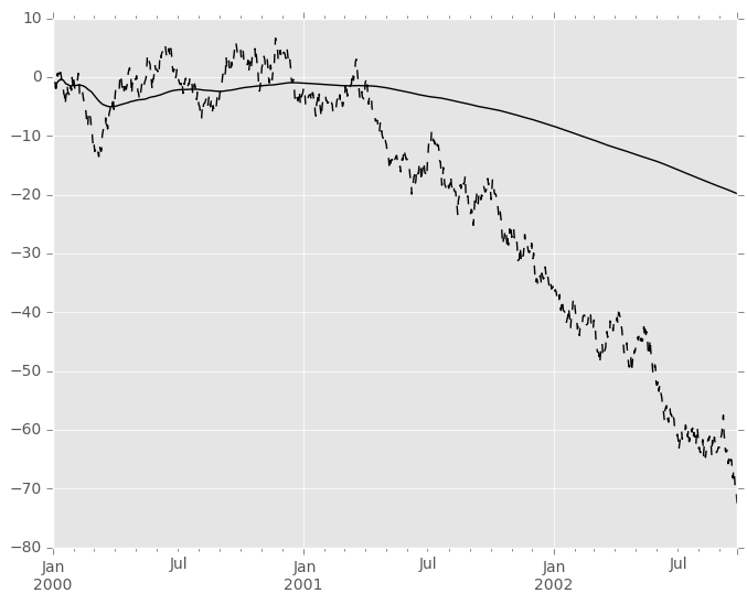
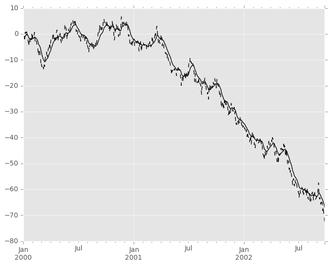
Here is an example for a univariate time series:

In [66]: plt.close('all')

In [67]: ts.plot(style='k--') Out[67]: <matplotlib.axes._subplots.AxesSubplot at 0xa9b1732c>

In [68]: pd.ewma(ts, span=20).plot(style='k') Out[68]: <matplotlib.axes._subplots.AxesSubplot at 0xa9b1732c>

_images/ewma_ex.png

All the EW functions have a min_periods argument, which has the same meaning it does for all the expanding_ and rolling_ functions: no output values will be set until at least min_periods non-null values are encountered in the (expanding) window. (This is a change from versions prior to 0.15.0, in which the min_periodsargument affected only the min_periods consecutive entries starting at the first non-null value.)

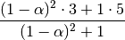
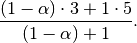
All the EW functions also have an ignore_na argument, which deterines how intermediate null values affect the calculation of the weights. When ignore_na=False (the default), weights are calculated based on absolute positions, so that intermediate null values affect the result. When ignore_na=True (which reproduces the behavior in versions prior to 0.15.0), weights are calculated by ignoring intermediate null values. For example, assuming adjust=True, if ignore_na=False, the weighted average of 3, NaN, 5 would be calculated as

$\frac{(1-\alpha)^2 \cdot 3 + 1 \cdot 5}{(1-\alpha)^2 + 1}$

Whereas if ignore_na=True, the weighted average would be calculated as

$\frac{(1-\alpha) \cdot 3 + 1 \cdot 5}{(1-\alpha) + 1}.$

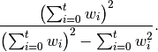
The ewmvar, ewmstd, and ewmcov functions have a bias argument, specifying whether the result should contain biased or unbiased statistics. For example, if bias=True, ewmvar(x) is calculated asewmvar(x) = ewma(x**2) - ewma(x)**2; whereas if bias=False (the default), the biased variance statistics are scaled by debiasing factors

$\frac{\left(\sum_{i=0}^t w_i\right)^2}{\left(\sum_{i=0}^t w_i\right)^2 - \sum_{i=0}^t w_i^2}.$

(For $w_i = 1$ , this reduces to the usual $N / (N - 1)$ factor, with $N = t + 1$ .) See http://en.wikipedia.org/wiki/Weighted_arithmetic_mean#Weighted_sample_variancefor further details.