Cookbook — pandas 0.16.2 documentation (original) (raw)
This is a repository for short and sweet examples and links for useful pandas recipes. We encourage users to add to this documentation.
Adding interesting links and/or inline examples to this section is a great First Pull Request.
Simplified, condensed, new-user friendly, in-line examples have been inserted where possible to augment the Stack-Overflow and GitHub links. Many of the links contain expanded information, above what the in-line examples offer.
Pandas (pd) and Numpy (np) are the only two abbreviated imported modules. The rest are kept explicitly imported for newer users.
These examples are written for python 3.4. Minor tweaks might be necessary for earlier python versions.
Idioms
These are some neat pandas idioms
if-then/if-then-else on one column, and assignment to another one or more columns:
In [1]: df = pd.DataFrame( ...: {'AAA' : [4,5,6,7], 'BBB' : [10,20,30,40],'CCC' : [100,50,-30,-50]}); df ...: Out[1]: AAA BBB CCC 0 4 10 100 1 5 20 50 2 6 30 -30 3 7 40 -50
if-then...
An if-then on one column
In [2]: df.ix[df.AAA >= 5,'BBB'] = -1; df Out[2]: AAA BBB CCC 0 4 10 100 1 5 -1 50 2 6 -1 -30 3 7 -1 -50
An if-then with assignment to 2 columns:
In [3]: df.ix[df.AAA >= 5,['BBB','CCC']] = 555; df Out[3]: AAA BBB CCC 0 4 10 100 1 5 555 555 2 6 555 555 3 7 555 555
Add another line with different logic, to do the -else
In [4]: df.ix[df.AAA < 5,['BBB','CCC']] = 2000; df Out[4]: AAA BBB CCC 0 4 2000 2000 1 5 555 555 2 6 555 555 3 7 555 555
Or use pandas where after you’ve set up a mask
In [5]: df_mask = pd.DataFrame({'AAA' : [True] * 4, 'BBB' : [False] * 4,'CCC' : [True,False] * 2})
In [6]: df.where(df_mask,-1000) Out[6]: AAA BBB CCC 0 4 -1000 2000 1 5 -1000 -1000 2 6 -1000 555 3 7 -1000 -1000
if-then-else using numpy’s where()
In [7]: df = pd.DataFrame( ...: {'AAA' : [4,5,6,7], 'BBB' : [10,20,30,40],'CCC' : [100,50,-30,-50]}); df ...: Out[7]: AAA BBB CCC 0 4 10 100 1 5 20 50 2 6 30 -30 3 7 40 -50
In [8]: df['logic'] = np.where(df['AAA'] > 5,'high','low'); df Out[8]: AAA BBB CCC logic 0 4 10 100 low 1 5 20 50 low 2 6 30 -30 high 3 7 40 -50 high
Splitting
Split a frame with a boolean criterion
In [9]: df = pd.DataFrame( ...: {'AAA' : [4,5,6,7], 'BBB' : [10,20,30,40],'CCC' : [100,50,-30,-50]}); df ...: Out[9]: AAA BBB CCC 0 4 10 100 1 5 20 50 2 6 30 -30 3 7 40 -50
In [10]: dflow = df[df.AAA <= 5]
In [11]: dfhigh = df[df.AAA > 5]
In [12]: dflow; dfhigh Out[12]: AAA BBB CCC 2 6 30 -30 3 7 40 -50
Building Criteria
Select with multi-column criteria
In [13]: df = pd.DataFrame( ....: {'AAA' : [4,5,6,7], 'BBB' : [10,20,30,40],'CCC' : [100,50,-30,-50]}); df ....: Out[13]: AAA BBB CCC 0 4 10 100 1 5 20 50 2 6 30 -30 3 7 40 -50
...and (without assignment returns a Series)
In [14]: newseries = df.loc[(df['BBB'] < 25) & (df['CCC'] >= -40), 'AAA']; newseries Out[14]: 0 4 1 5 Name: AAA, dtype: int64
...or (without assignment returns a Series)
In [15]: newseries = df.loc[(df['BBB'] > 25) | (df['CCC'] >= -40), 'AAA']; newseries;
...or (with assignment modifies the DataFrame.)
In [16]: df.loc[(df['BBB'] > 25) | (df['CCC'] >= 75), 'AAA'] = 0.1; df Out[16]: AAA BBB CCC 0 0.1 10 100 1 5.0 20 50 2 0.1 30 -30 3 0.1 40 -50
Select rows with data closest to certain value using argsort
In [17]: df = pd.DataFrame( ....: {'AAA' : [4,5,6,7], 'BBB' : [10,20,30,40],'CCC' : [100,50,-30,-50]}); df ....: Out[17]: AAA BBB CCC 0 4 10 100 1 5 20 50 2 6 30 -30 3 7 40 -50
In [18]: aValue = 43.0
In [19]: df.ix[(df.CCC-aValue).abs().argsort()] Out[19]: AAA BBB CCC 1 5 20 50 0 4 10 100 2 6 30 -30 3 7 40 -50
Dynamically reduce a list of criteria using a binary operators
In [20]: df = pd.DataFrame( ....: {'AAA' : [4,5,6,7], 'BBB' : [10,20,30,40],'CCC' : [100,50,-30,-50]}); df ....: Out[20]: AAA BBB CCC 0 4 10 100 1 5 20 50 2 6 30 -30 3 7 40 -50
In [21]: Crit1 = df.AAA <= 5.5
In [22]: Crit2 = df.BBB == 10.0
In [23]: Crit3 = df.CCC > -40.0
One could hard code:
In [24]: AllCrit = Crit1 & Crit2 & Crit3
...Or it can be done with a list of dynamically built criteria
In [25]: CritList = [Crit1,Crit2,Crit3]
In [26]: AllCrit = functools.reduce(lambda x,y: x & y, CritList)
In [27]: df[AllCrit] Out[27]: AAA BBB CCC 0 4 10 100
Selection
DataFrames
The indexing docs.
Using both row labels and value conditionals
In [28]: df = pd.DataFrame( ....: {'AAA' : [4,5,6,7], 'BBB' : [10,20,30,40],'CCC' : [100,50,-30,-50]}); df ....: Out[28]: AAA BBB CCC 0 4 10 100 1 5 20 50 2 6 30 -30 3 7 40 -50
In [29]: df[(df.AAA <= 6) & (df.index.isin([0,2,4]))] Out[29]: AAA BBB CCC 0 4 10 100 2 6 30 -30
Use loc for label-oriented slicing and iloc positional slicing
In [30]: data = {'AAA' : [4,5,6,7], 'BBB' : [10,20,30,40],'CCC' : [100,50,-30,-50]}
In [31]: df = pd.DataFrame(data=data,index=['foo','bar','boo','kar']); df Out[31]: AAA BBB CCC foo 4 10 100 bar 5 20 50 boo 6 30 -30 kar 7 40 -50
There are 2 explicit slicing methods, with a third general case
- Positional-oriented (Python slicing style : exclusive of end)
- Label-oriented (Non-Python slicing style : inclusive of end)
- General (Either slicing style : depends on if the slice contains labels or positions)
In [32]: df.loc['bar':'kar'] #Label Out[32]: AAA BBB CCC bar 5 20 50 boo 6 30 -30 kar 7 40 -50
#Generic In [33]: df.ix[0:3] #Same as .iloc[0:3] Out[33]: AAA BBB CCC foo 4 10 100 bar 5 20 50 boo 6 30 -30
In [34]: df.ix['bar':'kar'] #Same as .loc['bar':'kar'] Out[34]: AAA BBB CCC bar 5 20 50 boo 6 30 -30 kar 7 40 -50
Ambiguity arises when an index consists of integers with a non-zero start or non-unit increment.
In [35]: df2 = pd.DataFrame(data=data,index=[1,2,3,4]); #Note index starts at 1.
In [36]: df2.iloc[1:3] #Position-oriented Out[36]: AAA BBB CCC 2 5 20 50 3 6 30 -30
In [37]: df2.loc[1:3] #Label-oriented Out[37]: AAA BBB CCC 1 4 10 100 2 5 20 50 3 6 30 -30
In [38]: df2.ix[1:3] #General, will mimic loc (label-oriented) Out[38]: AAA BBB CCC 1 4 10 100 2 5 20 50 3 6 30 -30
In [39]: df2.ix[0:3] #General, will mimic iloc (position-oriented), as loc[0:3] would raise a KeyError Out[39]: AAA BBB CCC 1 4 10 100 2 5 20 50 3 6 30 -30
Using inverse operator (~) to take the complement of a mask
In [40]: df = pd.DataFrame( ....: {'AAA' : [4,5,6,7], 'BBB' : [10,20,30,40], 'CCC' : [100,50,-30,-50]}); df ....: Out[40]: AAA BBB CCC 0 4 10 100 1 5 20 50 2 6 30 -30 3 7 40 -50
In [41]: df[~((df.AAA <= 6) & (df.index.isin([0,2,4])))] Out[41]: AAA BBB CCC 1 5 20 50 3 7 40 -50
Panels
In [42]: rng = pd.date_range('1/1/2013',periods=100,freq='D')
In [43]: data = np.random.randn(100, 4)
In [44]: cols = ['A','B','C','D']
In [45]: df1, df2, df3 = pd.DataFrame(data, rng, cols), pd.DataFrame(data, rng, cols), pd.DataFrame(data, rng, cols)
In [46]: pf = pd.Panel({'df1':df1,'df2':df2,'df3':df3});pf Out[46]: <class 'pandas.core.panel.Panel'> Dimensions: 3 (items) x 100 (major_axis) x 4 (minor_axis) Items axis: df1 to df3 Major_axis axis: 2013-01-01 00:00:00 to 2013-04-10 00:00:00 Minor_axis axis: A to D
#Assignment using Transpose (pandas < 0.15) In [47]: pf = pf.transpose(2,0,1)
In [48]: pf['E'] = pd.DataFrame(data, rng, cols)
In [49]: pf = pf.transpose(1,2,0);pf Out[49]: <class 'pandas.core.panel.Panel'> Dimensions: 3 (items) x 100 (major_axis) x 5 (minor_axis) Items axis: df1 to df3 Major_axis axis: 2013-01-01 00:00:00 to 2013-04-10 00:00:00 Minor_axis axis: A to E
#Direct assignment (pandas > 0.15) In [50]: pf.loc[:,:,'F'] = pd.DataFrame(data, rng, cols);pf Out[50]: <class 'pandas.core.panel.Panel'> Dimensions: 3 (items) x 100 (major_axis) x 6 (minor_axis) Items axis: df1 to df3 Major_axis axis: 2013-01-01 00:00:00 to 2013-04-10 00:00:00 Minor_axis axis: A to F
Mask a panel by using np.where and then reconstructing the panel with the new masked values
New Columns
Efficiently and dynamically creating new columns using applymap
In [51]: df = pd.DataFrame( ....: {'AAA' : [1,2,1,3], 'BBB' : [1,1,2,2], 'CCC' : [2,1,3,1]}); df ....: Out[51]: AAA BBB CCC 0 1 1 2 1 2 1 1 2 1 2 3 3 3 2 1
In [52]: source_cols = df.columns # or some subset would work too.
In [53]: new_cols = [str(x) + "_cat" for x in source_cols]
In [54]: categories = {1 : 'Alpha', 2 : 'Beta', 3 : 'Charlie' }
In [55]: df[new_cols] = df[source_cols].applymap(categories.get);df Out[55]: AAA BBB CCC AAA_cat BBB_cat CCC_cat 0 1 1 2 Alpha Alpha Beta 1 2 1 1 Beta Alpha Alpha 2 1 2 3 Alpha Beta Charlie 3 3 2 1 Charlie Beta Alpha
Keep other columns when using min() with groupby
In [56]: df = pd.DataFrame( ....: {'AAA' : [1,1,1,2,2,2,3,3], 'BBB' : [2,1,3,4,5,1,2,3]}); df ....: Out[56]: AAA BBB 0 1 2 1 1 1 2 1 3 3 2 4 4 2 5 5 2 1 6 3 2 7 3 3
Method 1 : idxmin() to get the index of the mins
In [57]: df.loc[df.groupby("AAA")["BBB"].idxmin()] Out[57]: AAA BBB 1 1 1 5 2 1 6 3 2
Method 2 : sort then take first of each
In [58]: df.sort("BBB").groupby("AAA", as_index=False).first() Out[58]: AAA BBB 0 1 1 1 2 1 2 3 2
Notice the same results, with the exception of the index.
MultiIndexing
The multindexing docs.
Creating a multi-index from a labeled frame
In [59]: df = pd.DataFrame({'row' : [0,1,2], ....: 'One_X' : [1.1,1.1,1.1], ....: 'One_Y' : [1.2,1.2,1.2], ....: 'Two_X' : [1.11,1.11,1.11], ....: 'Two_Y' : [1.22,1.22,1.22]}); df ....: Out[59]: One_X One_Y Two_X Two_Y row 0 1.1 1.2 1.11 1.22 0 1 1.1 1.2 1.11 1.22 1 2 1.1 1.2 1.11 1.22 2
As Labelled Index
In [60]: df = df.set_index('row');df
Out[60]:
One_X One_Y Two_X Two_Y
row
0 1.1 1.2 1.11 1.22
1 1.1 1.2 1.11 1.22
2 1.1 1.2 1.11 1.22
With Heirarchical Columns
In [61]: df.columns = pd.MultiIndex.from_tuples([tuple(c.split('_')) for c in df.columns]);df
Out[61]:
One Two
X Y X Y
row
0 1.1 1.2 1.11 1.22
1 1.1 1.2 1.11 1.22
2 1.1 1.2 1.11 1.22
Now stack & Reset
In [62]: df = df.stack(0).reset_index(1);df
Out[62]:
level_1 X Y
row
0 One 1.10 1.20
0 Two 1.11 1.22
1 One 1.10 1.20
1 Two 1.11 1.22
2 One 1.10 1.20
2 Two 1.11 1.22
And fix the labels (Notice the label 'level_1' got added automatically)
In [63]: df.columns = ['Sample','All_X','All_Y'];df
Out[63]:
Sample All_X All_Y
row
0 One 1.10 1.20
0 Two 1.11 1.22
1 One 1.10 1.20
1 Two 1.11 1.22
2 One 1.10 1.20
2 Two 1.11 1.22
Arithmetic
Performing arithmetic with a multi-index that needs broadcasting
In [64]: cols = pd.MultiIndex.from_tuples([ (x,y) for x in ['A','B','C'] for y in ['O','I']])
In [65]: df = pd.DataFrame(np.random.randn(2,6),index=['n','m'],columns=cols); df
Out[65]:
A B C
O I O I O I
n 1.920906 -0.388231 -2.314394 0.665508 0.402562 0.399555
m -1.765956 0.850423 0.388054 0.992312 0.744086 -0.739776
In [66]: df = df.div(df['C'],level=1); df
Out[66]:
A B C
O I O I O I
n 4.771702 -0.971660 -5.749162 1.665625 1 1
m -2.373321 -1.149568 0.521518 -1.341367 1 1
Slicing
In [67]: coords = [('AA','one'),('AA','six'),('BB','one'),('BB','two'),('BB','six')]
In [68]: index = pd.MultiIndex.from_tuples(coords)
In [69]: df = pd.DataFrame([11,22,33,44,55],index,['MyData']); df Out[69]: MyData AA one 11 six 22 BB one 33 two 44 six 55
To take the cross section of the 1st level and 1st axis the index:
In [70]: df.xs('BB',level=0,axis=0) #Note : level and axis are optional, and default to zero Out[70]: MyData one 33 two 44 six 55
...and now the 2nd level of the 1st axis.
In [71]: df.xs('six',level=1,axis=0) Out[71]: MyData AA 22 BB 55
Slicing a multi-index with xs, method #2
In [72]: index = list(itertools.product(['Ada','Quinn','Violet'],['Comp','Math','Sci']))
In [73]: headr = list(itertools.product(['Exams','Labs'],['I','II']))
In [74]: indx = pd.MultiIndex.from_tuples(index,names=['Student','Course'])
In [75]: cols = pd.MultiIndex.from_tuples(headr) #Notice these are un-named
In [76]: data = [[70+x+y+(x*y)%3 for x in range(4)] for y in range(9)]
In [77]: df = pd.DataFrame(data,indx,cols); df
Out[77]:
Exams Labs
I II I II
Student Course
Ada Comp 70 71 72 73
Math 71 73 75 74
Sci 72 75 75 75
Quinn Comp 73 74 75 76
Math 74 76 78 77
Sci 75 78 78 78
Violet Comp 76 77 78 79
Math 77 79 81 80
Sci 78 81 81 81
In [78]: All = slice(None)
In [79]: df.loc['Violet']
Out[79]:
Exams Labs
I II I II
Course
Comp 76 77 78 79
Math 77 79 81 80
Sci 78 81 81 81
In [80]: df.loc[(All,'Math'),All]
Out[80]:
Exams Labs
I II I II
Student Course
Ada Math 71 73 75 74
Quinn Math 74 76 78 77
Violet Math 77 79 81 80
In [81]: df.loc[(slice('Ada','Quinn'),'Math'),All]
Out[81]:
Exams Labs
I II I II
Student Course
Ada Math 71 73 75 74
Quinn Math 74 76 78 77
In [82]: df.loc[(All,'Math'),('Exams')]
Out[82]:
I II
Student Course
Ada Math 71 73
Quinn Math 74 76
Violet Math 77 79
In [83]: df.loc[(All,'Math'),(All,'II')]
Out[83]:
Exams Labs
II II
Student Course
Ada Math 73 74
Quinn Math 76 77
Violet Math 79 80
Setting portions of a multi-index with xs
Missing Data
The missing data docs.
Fill forward a reversed timeseries
In [85]: df = pd.DataFrame(np.random.randn(6,1), index=pd.date_range('2013-08-01', periods=6, freq='B'), columns=list('A'))
In [86]: df.ix[3,'A'] = np.nan
In [87]: df Out[87]: A 2013-08-01 -1.054874 2013-08-02 -0.179642 2013-08-05 0.639589 2013-08-06 NaN 2013-08-07 1.906684 2013-08-08 0.104050
In [88]: df.reindex(df.index[::-1]).ffill() Out[88]: A 2013-08-08 0.104050 2013-08-07 1.906684 2013-08-06 1.906684 2013-08-05 0.639589 2013-08-02 -0.179642 2013-08-01 -1.054874
Grouping
The grouping docs.
Unlike agg, apply’s callable is passed a sub-DataFrame which gives you access to all the columns
In [89]: df = pd.DataFrame({'animal': 'cat dog cat fish dog cat cat'.split(), ....: 'size': list('SSMMMLL'), ....: 'weight': [8, 10, 11, 1, 20, 12, 12], ....: 'adult' : [False] * 5 + [True] * 2}); df ....: Out[89]: adult animal size weight 0 False cat S 8 1 False dog S 10 2 False cat M 11 3 False fish M 1 4 False dog M 20 5 True cat L 12 6 True cat L 12
#List the size of the animals with the highest weight. In [90]: df.groupby('animal').apply(lambda subf: subf['size'][subf['weight'].idxmax()]) Out[90]: animal cat L dog M fish M dtype: object
In [91]: gb = df.groupby(['animal'])
In [92]: gb.get_group('cat') Out[92]: adult animal size weight 0 False cat S 8 2 False cat M 11 5 True cat L 12 6 True cat L 12
Apply to different items in a group
In [93]: def GrowUp(x): ....: avg_weight = sum(x[x['size'] == 'S'].weight * 1.5) ....: avg_weight += sum(x[x['size'] == 'M'].weight * 1.25) ....: avg_weight += sum(x[x['size'] == 'L'].weight) ....: avg_weight /= len(x) ....: return pd.Series(['L',avg_weight,True], index=['size', 'weight', 'adult']) ....:
In [94]: expected_df = gb.apply(GrowUp)
In [95]: expected_df
Out[95]:
size weight adult
animal
cat L 12.4375 True
dog L 20.0000 True
fish L 1.2500 True
In [96]: S = pd.Series([i / 100.0 for i in range(1,11)])
In [97]: def CumRet(x,y): ....: return x * (1 + y) ....:
In [98]: def Red(x): ....: return functools.reduce(CumRet,x,1.0) ....:
In [99]: pd.expanding_apply(S, Red) Out[99]: 0 1.010000 1 1.030200 2 1.061106 3 1.103550 4 1.158728 5 1.228251 6 1.314229 7 1.419367 8 1.547110 9 1.701821 dtype: float64
Replacing some values with mean of the rest of a group
In [100]: df = pd.DataFrame({'A' : [1, 1, 2, 2], 'B' : [1, -1, 1, 2]})
In [101]: gb = df.groupby('A')
In [102]: def replace(g): .....: mask = g < 0 .....: g.loc[mask] = g[~mask].mean() .....: return g .....:
In [103]: gb.transform(replace) Out[103]: B 0 1 1 1 2 1 3 2
Sort groups by aggregated data
In [104]: df = pd.DataFrame({'code': ['foo', 'bar', 'baz'] * 2, .....: 'data': [0.16, -0.21, 0.33, 0.45, -0.59, 0.62], .....: 'flag': [False, True] * 3}) .....:
In [105]: code_groups = df.groupby('code')
In [106]: agg_n_sort_order = code_groups[['data']].transform(sum).sort('data')
In [107]: sorted_df = df.ix[agg_n_sort_order.index]
In [108]: sorted_df Out[108]: code data flag 1 bar -0.21 True 4 bar -0.59 False 0 foo 0.16 False 3 foo 0.45 True 2 baz 0.33 False 5 baz 0.62 True
Create multiple aggregated columns
In [109]: rng = pd.date_range(start="2014-10-07",periods=10,freq='2min')
In [110]: ts = pd.Series(data = list(range(10)), index = rng)
In [111]: def MyCust(x): .....: if len(x) > 2: .....: return x[1] * 1.234 .....: return pd.NaT .....:
In [112]: mhc = {'Mean' : np.mean, 'Max' : np.max, 'Custom' : MyCust}
In [113]: ts.resample("5min",how = mhc) Out[113]: Max Custom Mean 2014-10-07 00:00:00 2 1.234 1.0 2014-10-07 00:05:00 4 NaN 3.5 2014-10-07 00:10:00 7 7.404 6.0 2014-10-07 00:15:00 9 NaN 8.5
In [114]: ts Out[114]: 2014-10-07 00:00:00 0 2014-10-07 00:02:00 1 2014-10-07 00:04:00 2 2014-10-07 00:06:00 3 2014-10-07 00:08:00 4 2014-10-07 00:10:00 5 2014-10-07 00:12:00 6 2014-10-07 00:14:00 7 2014-10-07 00:16:00 8 2014-10-07 00🔞00 9 Freq: 2T, dtype: int64
Create a value counts column and reassign back to the DataFrame
In [115]: df = pd.DataFrame({'Color': 'Red Red Red Blue'.split(), .....: 'Value': [100, 150, 50, 50]}); df .....: Out[115]: Color Value 0 Red 100 1 Red 150 2 Red 50 3 Blue 50
In [116]: df['Counts'] = df.groupby(['Color']).transform(len)
In [117]: df Out[117]: Color Value Counts 0 Red 100 3 1 Red 150 3 2 Red 50 3 3 Blue 50 1
Shift groups of the values in a column based on the index
In [118]: df = pd.DataFrame( .....: {u'line_race': [10, 10, 8, 10, 10, 8], .....: u'beyer': [99, 102, 103, 103, 88, 100]}, .....: index=[u'Last Gunfighter', u'Last Gunfighter', u'Last Gunfighter', .....: u'Paynter', u'Paynter', u'Paynter']); df .....: Out[118]: beyer line_race Last Gunfighter 99 10 Last Gunfighter 102 10 Last Gunfighter 103 8 Paynter 103 10 Paynter 88 10 Paynter 100 8
In [119]: df['beyer_shifted'] = df.groupby(level=0)['beyer'].shift(1)
In [120]: df Out[120]: beyer line_race beyer_shifted Last Gunfighter 99 10 NaN Last Gunfighter 102 10 99 Last Gunfighter 103 8 102 Paynter 103 10 NaN Paynter 88 10 103 Paynter 100 8 88
Select row with maximum value from each group
In [121]: df = pd.DataFrame({'host':['other','other','that','this','this'], .....: 'service':['mail','web','mail','mail','web'], .....: 'no':[1, 2, 1, 2, 1]}).set_index(['host', 'service']) .....:
In [122]: mask = df.groupby(level=0).agg('idxmax')
In [123]: df_count = df.loc[mask['no']].reset_index()
In [124]: df_count Out[124]: host service no 0 other web 2 1 that mail 1 2 this mail 2
Grouping like Python’s itertools.groupby
In [125]: df = pd.DataFrame([0, 1, 0, 1, 1, 1, 0, 1, 1], columns=['A'])
In [126]: df.A.groupby((df.A != df.A.shift()).cumsum()).groups Out[126]: {1: [0L], 2: [1L], 3: [2L], 4: [3L, 4L, 5L], 5: [6L], 6: [7L, 8L]}
In [127]: df.A.groupby((df.A != df.A.shift()).cumsum()).cumsum() Out[127]: 0 0 1 1 2 0 3 1 4 2 5 3 6 0 7 1 8 2 dtype: int64
Splitting
Create a list of dataframes, split using a delineation based on logic included in rows.
In [128]: df = pd.DataFrame(data={'Case' : ['A','A','A','B','A','A','B','A','A'], .....: 'Data' : np.random.randn(9)}) .....:
In [129]: dfs = list(zip(df.groupby(pd.rolling_median((1(df['Case']=='B')).cumsum(),3,True))))[-1]
In [130]: dfs[0] Out[130]: Case Data 0 A 0.174068 1 A -0.439461 2 A -0.741343 3 B -0.079673
In [131]: dfs[1] Out[131]: Case Data 4 A -0.922875 5 A 0.303638 6 B -0.917368
In [132]: dfs[2] Out[132]: Case Data 7 A -1.624062 8 A -0.758514
Pivot
The Pivot docs.
In [133]: df = pd.DataFrame(data={'Province' : ['ON','QC','BC','AL','AL','MN','ON'], .....: 'City' : ['Toronto','Montreal','Vancouver','Calgary','Edmonton','Winnipeg','Windsor'], .....: 'Sales' : [13,6,16,8,4,3,1]}) .....:
In [134]: table = pd.pivot_table(df,values=['Sales'],index=['Province'],columns=['City'],aggfunc=np.sum,margins=True)
In [135]: table.stack('City')
Out[135]:
Sales
Province City
AL All 12
Calgary 8
Edmonton 4
BC All 16
Vancouver 16
MN All 3
Winnipeg 3
... ...
All Calgary 8
Edmonton 4
Montreal 6
Toronto 13
Vancouver 16
Windsor 1
Winnipeg 3
[20 rows x 1 columns]
Frequency table like plyr in R
In [136]: grades = [48,99,75,80,42,80,72,68,36,78]
In [137]: df = pd.DataFrame( {'ID': ["x%d" % r for r in range(10)], .....: 'Gender' : ['F', 'M', 'F', 'M', 'F', 'M', 'F', 'M', 'M', 'M'], .....: 'ExamYear': ['2007','2007','2007','2008','2008','2008','2008','2009','2009','2009'], .....: 'Class': ['algebra', 'stats', 'bio', 'algebra', 'algebra', 'stats', 'stats', 'algebra', 'bio', 'bio'], .....: 'Participated': ['yes','yes','yes','yes','no','yes','yes','yes','yes','yes'], .....: 'Passed': ['yes' if x > 50 else 'no' for x in grades], .....: 'Employed': [True,True,True,False,False,False,False,True,True,False], .....: 'Grade': grades}) .....:
In [138]: df.groupby('ExamYear').agg({'Participated': lambda x: x.value_counts()['yes'],
.....: 'Passed': lambda x: sum(x == 'yes'),
.....: 'Employed' : lambda x : sum(x),
.....: 'Grade' : lambda x : sum(x) / len(x)})
.....:
Out[138]:
Grade Employed Participated Passed
ExamYear
2007 74 3 3 2
2008 68 0 3 3
2009 60 2 3 2
Apply
Rolling Apply to Organize - Turning embedded lists into a multi-index frame
In [139]: df = pd.DataFrame(data={'A' : [[2,4,8,16],[100,200],[10,20,30]], 'B' : [['a','b','c'],['jj','kk'],['ccc']]},index=['I','II','III'])
In [140]: def SeriesFromSubList(aList): .....: return pd.Series(aList) .....:
In [141]: df_orgz = pd.concat(dict([ (ind,row.apply(SeriesFromSubList)) for ind,row in df.iterrows() ]))
Rolling Apply with a DataFrame returning a Series
Rolling Apply to multiple columns where function calculates a Series before a Scalar from the Series is returned
In [142]: df = pd.DataFrame(data=np.random.randn(2000,2)/10000, .....: index=pd.date_range('2001-01-01',periods=2000), .....: columns=['A','B']); df .....: Out[142]: A B 2001-01-01 -0.000056 -0.000059 2001-01-02 -0.000107 -0.000168 2001-01-03 0.000040 0.000061 2001-01-04 0.000039 0.000182 2001-01-05 0.000071 -0.000067 2001-01-06 0.000024 0.000031 2001-01-07 0.000012 -0.000021 ... ... ... 2006-06-17 0.000129 0.000094 2006-06-18 0.000059 0.000216 2006-06-19 -0.000069 0.000283 2006-06-20 0.000089 0.000084 2006-06-21 0.000075 0.000041 2006-06-22 -0.000037 -0.000011 2006-06-23 -0.000070 -0.000048
[2000 rows x 2 columns]
In [143]: def gm(aDF,Const): .....: v = ((((aDF.A+aDF.B)+1).cumprod())-1)*Const .....: return (aDF.index[0],v.iloc[-1]) .....:
In [144]: S = pd.Series(dict([ gm(df.iloc[i:min(i+51,len(df)-1)],5) for i in range(len(df)-50) ])); S
Out[144]:
2001-01-01 -0.003108
2001-01-02 -0.001787
2001-01-03 0.000204
2001-01-04 -0.000166
2001-01-05 -0.002148
2001-01-06 -0.001831
2001-01-07 -0.001663
...
2006-04-28 -0.009152
2006-04-29 -0.006728
2006-04-30 -0.005840
2006-05-01 -0.003650
2006-05-02 -0.003801
2006-05-03 -0.004272
2006-05-04 -0.003839
dtype: float64
Rolling apply with a DataFrame returning a Scalar
Rolling Apply to multiple columns where function returns a Scalar (Volume Weighted Average Price)
In [145]: rng = pd.date_range(start = '2014-01-01',periods = 100)
In [146]: df = pd.DataFrame({'Open' : np.random.randn(len(rng)), .....: 'Close' : np.random.randn(len(rng)), .....: 'Volume' : np.random.randint(100,2000,len(rng))}, index=rng); df .....: Out[146]: Close Open Volume 2014-01-01 1.550590 0.458513 1371 2014-01-02 -0.818812 -0.508850 1433 2014-01-03 1.160619 0.257610 645 2014-01-04 0.081521 -1.773393 878 2014-01-05 1.083284 -0.560676 1143 2014-01-06 -0.518721 0.284174 1088 2014-01-07 0.140661 1.146889 1722 ... ... ... ... 2014-04-04 0.458193 -0.669474 1768 2014-04-05 0.108502 -1.616315 836 2014-04-06 1.418082 -1.294906 694 2014-04-07 0.486530 1.171647 796 2014-04-08 0.181885 0.501639 265 2014-04-09 -0.707238 -0.361868 1293 2014-04-10 1.211432 1.564429 1088
[100 rows x 3 columns]
In [147]: def vwap(bars): return ((bars.Close*bars.Volume).sum()/bars.Volume.sum()).round(2)
In [148]: window = 5
In [149]: s = pd.concat([ (pd.Series(vwap(df.iloc[i:i+window]), index=[df.index[i+window]])) for i in range(len(df)-window) ]); s Out[149]: 2014-01-06 0.55 2014-01-07 0.06 2014-01-08 0.32 2014-01-09 0.03 2014-01-10 0.08 2014-01-11 -0.50 2014-01-12 -0.26 ... 2014-04-04 0.36 2014-04-05 0.48 2014-04-06 0.54 2014-04-07 0.46 2014-04-08 0.45 2014-04-09 0.53 2014-04-10 0.15 dtype: float64
Merge
The Concat docs. The Join docs.
Append two dataframes with overlapping index (emulate R rbind)
In [152]: rng = pd.date_range('2000-01-01', periods=6)
In [153]: df1 = pd.DataFrame(np.random.randn(6, 3), index=rng, columns=['A', 'B', 'C'])
In [154]: df2 = df1.copy()
ignore_index is needed in pandas < v0.13, and depending on df construction
In [155]: df = df1.append(df2,ignore_index=True); df Out[155]: A B C 0 -0.174202 -0.477257 0.239870 1 -0.654455 -1.411456 -1.778457 2 0.351578 0.307871 -0.286865 3 0.565398 -0.185821 0.937593 4 0.446473 0.566368 0.721476 5 1.710685 -0.667054 -0.651191 6 -0.174202 -0.477257 0.239870 7 -0.654455 -1.411456 -1.778457 8 0.351578 0.307871 -0.286865 9 0.565398 -0.185821 0.937593 10 0.446473 0.566368 0.721476 11 1.710685 -0.667054 -0.651191
In [156]: df = pd.DataFrame(data={'Area' : ['A'] * 5 + ['C'] * 2, .....: 'Bins' : [110] * 2 + [160] * 3 + [40] * 2, .....: 'Test_0' : [0, 1, 0, 1, 2, 0, 1], .....: 'Data' : np.random.randn(7)});df .....: Out[156]: Area Bins Data Test_0 0 A 110 -0.399974 0 1 A 110 -1.519206 1 2 A 160 1.678487 0 3 A 160 0.005345 1 4 A 160 -0.534461 2 5 C 40 0.255077 0 6 C 40 1.093310 1
In [157]: df['Test_1'] = df['Test_0'] - 1
In [158]: pd.merge(df, df, left_on=['Bins', 'Area','Test_0'], right_on=['Bins', 'Area','Test_1'],suffixes=('_L','_R')) Out[158]: Area Bins Data_L Test_0_L Test_1_L Data_R Test_0_R Test_1_R 0 A 110 -0.399974 0 -1 -1.519206 1 0 1 A 160 1.678487 0 -1 0.005345 1 0 2 A 160 0.005345 1 0 -0.534461 2 1 3 C 40 0.255077 0 -1 1.093310 1 0
Join with a criteria based on the values
Plotting
The Plotting docs.
Setting x-axis major and minor labels
Plotting multiple charts in an ipython notebook
Annotate a time-series plot #2
Generate Embedded plots in excel files using Pandas, Vincent and xlsxwriter
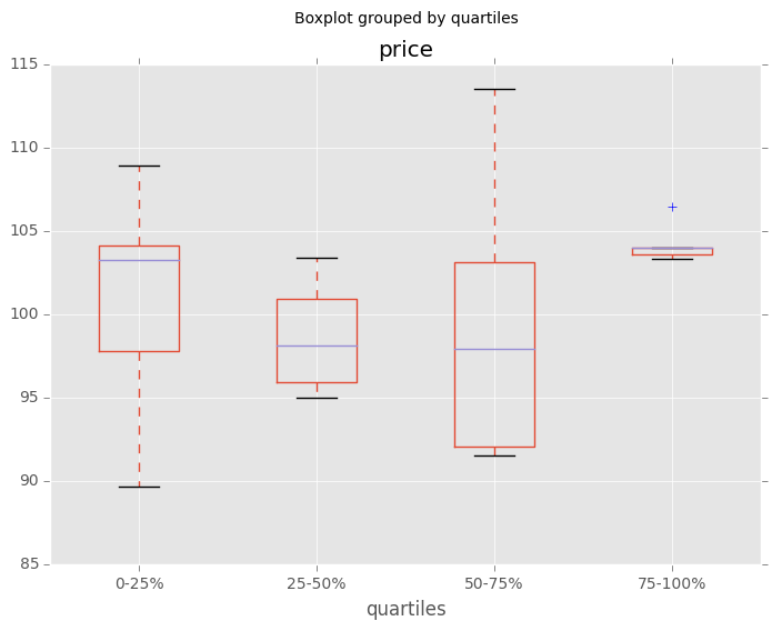
Boxplot for each quartile of a stratifying variable
In [159]: df = pd.DataFrame( .....: {u'stratifying_var': np.random.uniform(0, 100, 20), .....: u'price': np.random.normal(100, 5, 20)}) .....:
In [160]: df[u'quartiles'] = pd.qcut( .....: df[u'stratifying_var'], .....: 4, .....: labels=[u'0-25%', u'25-50%', u'50-75%', u'75-100%']) .....:
In [161]: df.boxplot(column=u'price', by=u'quartiles') Out[161]: <matplotlib.axes._subplots.AxesSubplot at 0xa98ad08c>
Data In/Out
Performance comparison of SQL vs HDF5
CSV
The CSV docs
how to read in multiple files, appending to create a single dataframe
Reading only certain rows of a csv chunk-by-chunk
Reading the first few lines of a frame
Reading a file that is compressed but not by gzip/bz2 (the native compressed formats which read_csv understands). This example shows a WinZipped file, but is a general application of opening the file within a context manager and using that handle to read.See here
Reading CSV with Unix timestamps and converting to local timezone
Write a multi-row index CSV without writing duplicates
Parsing date components in multi-columns is faster with a format
In [30]: i = pd.date_range('20000101',periods=10000)
In [31]: df = pd.DataFrame(dict(year = i.year, month = i.month, day = i.day))
In [32]: df.head() Out[32]: day month year 0 1 1 2000 1 2 1 2000 2 3 1 2000 3 4 1 2000 4 5 1 2000
In [33]: %timeit pd.to_datetime(df.year10000+df.month100+df.day,format='%Y%m%d') 100 loops, best of 3: 7.08 ms per loop
simulate combinging into a string, then parsing
In [34]: ds = df.apply(lambda x: "%04d%02d%02d" % (x['year'],x['month'],x['day']),axis=1)
In [35]: ds.head() Out[35]: 0 20000101 1 20000102 2 20000103 3 20000104 4 20000105 dtype: object
In [36]: %timeit pd.to_datetime(ds) 1 loops, best of 3: 488 ms per loop
Binary Files
pandas readily accepts numpy record arrays, if you need to read in a binary file consisting of an array of C structs. For example, given this C program in a file called main.c compiled with gcc main.c -std=gnu99 on a 64-bit machine,
#include <stdio.h> #include <stdint.h>
typedef struct _Data { int32_t count; double avg; float scale; } Data;
int main(int argc, const char *argv[]) { size_t n = 10; Data d[n];
for (int i = 0; i < n; ++i)
{
    d[i].count = i;
    d[i].avg = i + 1.0;
    d[i].scale = (float) i + 2.0f;
}

FILE *file = fopen("binary.dat", "wb");
fwrite(&d, sizeof(Data), n, file);
fclose(file);

return 0;
}
the following Python code will read the binary file 'binary.dat' into a pandas DataFrame, where each element of the struct corresponds to a column in the frame:
names = 'count', 'avg', 'scale'
note that the offsets are larger than the size of the type because of
struct padding
offsets = 0, 8, 16 formats = 'i4', 'f8', 'f4' dt = np.dtype({'names': names, 'offsets': offsets, 'formats': formats}, align=True) df = pd.DataFrame(np.fromfile('binary.dat', dt))
Note
The offsets of the structure elements may be different depending on the architecture of the machine on which the file was created. Using a raw binary file format like this for general data storage is not recommended, as it is not cross platform. We recommended either HDF5 or msgpack, both of which are supported by pandas’ IO facilities.
Timedeltas
The Timedeltas docs.
In [167]: s = pd.Series(pd.date_range('2012-1-1', periods=3, freq='D'))
In [168]: s - s.max() Out[168]: 0 -2 days 1 -1 days 2 0 days dtype: timedelta64[ns]
In [169]: s.max() - s Out[169]: 0 2 days 1 1 days 2 0 days dtype: timedelta64[ns]
In [170]: s - datetime.datetime(2011,1,1,3,5) Out[170]: 0 364 days 20:55:00 1 365 days 20:55:00 2 366 days 20:55:00 dtype: timedelta64[ns]
In [171]: s + datetime.timedelta(minutes=5) Out[171]: 0 2012-01-01 00:05:00 1 2012-01-02 00:05:00 2 2012-01-03 00:05:00 dtype: datetime64[ns]
In [172]: datetime.datetime(2011,1,1,3,5) - s Out[172]: 0 -365 days +03:05:00 1 -366 days +03:05:00 2 -367 days +03:05:00 dtype: timedelta64[ns]
In [173]: datetime.timedelta(minutes=5) + s Out[173]: 0 2012-01-01 00:05:00 1 2012-01-02 00:05:00 2 2012-01-03 00:05:00 dtype: datetime64[ns]
Adding and subtracting deltas and dates
In [174]: deltas = pd.Series([ datetime.timedelta(days=i) for i in range(3) ])
In [175]: df = pd.DataFrame(dict(A = s, B = deltas)); df Out[175]: A B 0 2012-01-01 0 days 1 2012-01-02 1 days 2 2012-01-03 2 days
In [176]: df['New Dates'] = df['A'] + df['B'];
In [177]: df['Delta'] = df['A'] - df['New Dates']; df Out[177]: A B New Dates Delta 0 2012-01-01 0 days 2012-01-01 0 days 1 2012-01-02 1 days 2012-01-03 -1 days 2 2012-01-03 2 days 2012-01-05 -2 days
In [178]: df.dtypes Out[178]: A datetime64[ns] B timedelta64[ns] New Dates datetime64[ns] Delta timedelta64[ns] dtype: object
Values can be set to NaT using np.nan, similar to datetime
In [179]: y = s - s.shift(); y Out[179]: 0 NaT 1 1 days 2 1 days dtype: timedelta64[ns]
In [180]: y[1] = np.nan; y Out[180]: 0 NaT 1 NaT 2 1 days dtype: timedelta64[ns]
Aliasing Axis Names
To globally provide aliases for axis names, one can define these 2 functions:
In [181]: def set_axis_alias(cls, axis, alias): .....: if axis not in cls._AXIS_NUMBERS: .....: raise Exception("invalid axis [%s] for alias [%s]" % (axis, alias)) .....: cls._AXIS_ALIASES[alias] = axis .....:
In [182]: def clear_axis_alias(cls, axis, alias): .....: if axis not in cls._AXIS_NUMBERS: .....: raise Exception("invalid axis [%s] for alias [%s]" % (axis, alias)) .....: cls._AXIS_ALIASES.pop(alias,None) .....:
In [183]: set_axis_alias(pd.DataFrame,'columns', 'myaxis2')
In [184]: df2 = pd.DataFrame(np.random.randn(3,2),columns=['c1','c2'],index=['i1','i2','i3'])
In [185]: df2.sum(axis='myaxis2') Out[185]: i1 0.239786 i2 0.259018 i3 0.163470 dtype: float64
In [186]: clear_axis_alias(pd.DataFrame,'columns', 'myaxis2')
Creating Example Data
To create a dataframe from every combination of some given values, like R’s expand.grid()function, we can create a dict where the keys are column names and the values are lists of the data values:
In [187]: def expand_grid(data_dict): .....: rows = itertools.product(*data_dict.values()) .....: return pd.DataFrame.from_records(rows, columns=data_dict.keys()) .....:
In [188]: df = expand_grid( .....: {'height': [60, 70], .....: 'weight': [100, 140, 180], .....: 'sex': ['Male', 'Female']}) .....:
In [189]: df Out[189]: sex weight height 0 Male 100 60 1 Male 100 70 2 Male 140 60 3 Male 140 70 4 Male 180 60 5 Male 180 70 6 Female 100 60 7 Female 100 70 8 Female 140 60 9 Female 140 70 10 Female 180 60 11 Female 180 70