Computational tools — pandas 0.24.0rc1 documentation (original) (raw)
Statistical Functions
Percent Change
Series, DataFrame, and Panel all have a methodpct_change() to compute the percent change over a given number of periods (using fill_method to fill NA/null values before computing the percent change).
In [1]: ser = pd.Series(np.random.randn(8))
In [2]: ser.pct_change() Out[2]: 0 NaN 1 -1.602976 2 4.334938 3 -0.247456 4 -2.067345 5 -1.142903 6 -1.688214 7 -9.759729 dtype: float64
In [3]: df = pd.DataFrame(np.random.randn(10, 4))
In [4]: df.pct_change(periods=3) Out[4]: 0 1 2 3 0 NaN NaN NaN NaN 1 NaN NaN NaN NaN 2 NaN NaN NaN NaN 3 -0.218320 -1.054001 1.987147 -0.510183 4 -0.439121 -1.816454 0.649715 -4.822809 5 -0.127833 -3.042065 -5.866604 -1.776977 6 -2.596833 -1.959538 -2.111697 -3.798900 7 -0.117826 -2.169058 0.036094 -0.067696 8 2.492606 -1.357320 -1.205802 -1.558697 9 -1.012977 2.324558 -1.003744 -0.371806
Covariance
Series.cov() can be used to compute covariance between series (excluding missing values).
In [5]: s1 = pd.Series(np.random.randn(1000))
In [6]: s2 = pd.Series(np.random.randn(1000))
In [7]: s1.cov(s2) Out[7]: 0.00068010881743108204
Analogously, DataFrame.cov() to compute pairwise covariances among the series in the DataFrame, also excluding NA/null values.
Note
Assuming the missing data are missing at random this results in an estimate for the covariance matrix which is unbiased. However, for many applications this estimate may not be acceptable because the estimated covariance matrix is not guaranteed to be positive semi-definite. This could lead to estimated correlations having absolute values which are greater than one, and/or a non-invertible covariance matrix. See Estimation of covariance matricesfor more details.
In [8]: frame = pd.DataFrame(np.random.randn(1000, 5), ...: columns=['a', 'b', 'c', 'd', 'e']) ...:
In [9]: frame.cov() Out[9]: a b c d e a 1.000882 -0.003177 -0.002698 -0.006889 0.031912 b -0.003177 1.024721 0.000191 0.009212 0.000857 c -0.002698 0.000191 0.950735 -0.031743 -0.005087 d -0.006889 0.009212 -0.031743 1.002983 -0.047952 e 0.031912 0.000857 -0.005087 -0.047952 1.042487
DataFrame.cov also supports an optional min_periods keyword that specifies the required minimum number of observations for each column pair in order to have a valid result.
In [10]: frame = pd.DataFrame(np.random.randn(20, 3), columns=['a', 'b', 'c'])
In [11]: frame.loc[frame.index[:5], 'a'] = np.nan
In [12]: frame.loc[frame.index[5:10], 'b'] = np.nan
In [13]: frame.cov() Out[13]: a b c a 1.123670 -0.412851 0.018169 b -0.412851 1.154141 0.305260 c 0.018169 0.305260 1.301149
In [14]: frame.cov(min_periods=12) Out[14]: a b c a 1.123670 NaN 0.018169 b NaN 1.154141 0.305260 c 0.018169 0.305260 1.301149
Correlation
Correlation may be computed using the corr() method. Using the method parameter, several methods for computing correlations are provided:
| Method name | Description |
|---|---|
| pearson (default) | Standard correlation coefficient |
| kendall | Kendall Tau correlation coefficient |
| spearman | Spearman rank correlation coefficient |
All of these are currently computed using pairwise complete observations. Wikipedia has articles covering the above correlation coefficients:
- Pearson correlation coefficient
- Kendall rank correlation coefficient
- Spearman’s rank correlation coefficient
Note
Please see the caveats associated with this method of calculating correlation matrices in thecovariance section.
In [15]: frame = pd.DataFrame(np.random.randn(1000, 5), ....: columns=['a', 'b', 'c', 'd', 'e']) ....:
In [16]: frame.iloc[::2] = np.nan
Series with Series
In [17]: frame['a'].corr(frame['b']) Out[17]: 0.013479040400098794
In [18]: frame['a'].corr(frame['b'], method='spearman') Out[18]: -0.0072898851595406371
Pairwise correlation of DataFrame columns
In [19]: frame.corr() Out[19]: a b c d e a 1.000000 0.013479 -0.049269 -0.042239 -0.028525 b 0.013479 1.000000 -0.020433 -0.011139 0.005654 c -0.049269 -0.020433 1.000000 0.018587 -0.054269 d -0.042239 -0.011139 0.018587 1.000000 -0.017060 e -0.028525 0.005654 -0.054269 -0.017060 1.000000
Note that non-numeric columns will be automatically excluded from the correlation calculation.
Like cov, corr also supports the optional min_periods keyword:
In [20]: frame = pd.DataFrame(np.random.randn(20, 3), columns=['a', 'b', 'c'])
In [21]: frame.loc[frame.index[:5], 'a'] = np.nan
In [22]: frame.loc[frame.index[5:10], 'b'] = np.nan
In [23]: frame.corr() Out[23]: a b c a 1.000000 -0.121111 0.069544 b -0.121111 1.000000 0.051742 c 0.069544 0.051742 1.000000
In [24]: frame.corr(min_periods=12) Out[24]: a b c a 1.000000 NaN 0.069544 b NaN 1.000000 0.051742 c 0.069544 0.051742 1.000000
New in version 0.24.0.
The method argument can also be a callable for a generic correlation calculation. In this case, it should be a single function that produces a single value from two ndarray inputs. Suppose we wanted to compute the correlation based on histogram intersection:
histogram intersection
In [25]: def histogram_intersection(a, b): ....: return np.minimum(np.true_divide(a, a.sum()), ....: np.true_divide(b, b.sum())).sum() ....:
In [26]: frame.corr(method=histogram_intersection) Out[26]: a b c a 1.000000 -6.404882 -2.058431 b -6.404882 1.000000 -19.255743 c -2.058431 -19.255743 1.000000
A related method corrwith() is implemented on DataFrame to compute the correlation between like-labeled Series contained in different DataFrame objects.
In [27]: index = ['a', 'b', 'c', 'd', 'e']
In [28]: columns = ['one', 'two', 'three', 'four']
In [29]: df1 = pd.DataFrame(np.random.randn(5, 4), index=index, columns=columns)
In [30]: df2 = pd.DataFrame(np.random.randn(4, 4), index=index[:4], columns=columns)
In [31]: df1.corrwith(df2) Out[31]: one -0.125501 two -0.493244 three 0.344056 four 0.004183 dtype: float64
In [32]: df2.corrwith(df1, axis=1) Out[32]: a -0.675817 b 0.458296 c 0.190809 d -0.186275 e NaN dtype: float64
Data ranking
The rank() method produces a data ranking with ties being assigned the mean of the ranks (by default) for the group:
In [33]: s = pd.Series(np.random.np.random.randn(5), index=list('abcde'))
In [34]: s['d'] = s['b'] # so there's a tie
In [35]: s.rank() Out[35]: a 5.0 b 2.5 c 1.0 d 2.5 e 4.0 dtype: float64
rank() is also a DataFrame method and can rank either the rows (axis=0) or the columns (axis=1). NaN values are excluded from the ranking.
In [36]: df = pd.DataFrame(np.random.np.random.randn(10, 6))
In [37]: df[4] = df[2][:5] # some ties
In [38]: df Out[38]: 0 1 2 3 4 5 0 -0.904948 -1.163537 -1.457187 0.135463 -1.457187 0.294650 1 -0.976288 -0.244652 -0.748406 -0.999601 -0.748406 -0.800809 2 0.401965 1.460840 1.256057 1.308127 1.256057 0.876004 3 0.205954 0.369552 -0.669304 0.038378 -0.669304 1.140296 4 -0.477586 -0.730705 -1.129149 -0.601463 -1.129149 -0.211196 5 -1.092970 -0.689246 0.908114 0.204848 NaN 0.463347 6 0.376892 0.959292 0.095572 -0.593740 NaN -0.069180 7 -1.002601 1.957794 -0.120708 0.094214 NaN -1.467422 8 -0.547231 0.664402 -0.519424 -0.073254 NaN -1.263544 9 -0.250277 -0.237428 -1.056443 0.419477 NaN 1.375064
In [39]: df.rank(1) Out[39]: 0 1 2 3 4 5 0 4.0 3.0 1.5 5.0 1.5 6.0 1 2.0 6.0 4.5 1.0 4.5 3.0 2 1.0 6.0 3.5 5.0 3.5 2.0 3 4.0 5.0 1.5 3.0 1.5 6.0 4 5.0 3.0 1.5 4.0 1.5 6.0 5 1.0 2.0 5.0 3.0 NaN 4.0 6 4.0 5.0 3.0 1.0 NaN 2.0 7 2.0 5.0 3.0 4.0 NaN 1.0 8 2.0 5.0 3.0 4.0 NaN 1.0 9 2.0 3.0 1.0 4.0 NaN 5.0
rank optionally takes a parameter ascending which by default is true; when false, data is reverse-ranked, with larger values assigned a smaller rank.
rank supports different tie-breaking methods, specified with the methodparameter:
average: average rank of tied groupmin: lowest rank in the groupmax: highest rank in the groupfirst: ranks assigned in the order they appear in the array
Window Functions
For working with data, a number of window functions are provided for computing common window or rolling statistics. Among these are count, sum, mean, median, correlation, variance, covariance, standard deviation, skewness, and kurtosis.
The rolling() and expanding()functions can be used directly from DataFrameGroupBy objects, see the groupby docs.
Note
The API for window statistics is quite similar to the way one works with GroupBy objects, see the documentation here.
We work with rolling, expanding and exponentially weighted data through the corresponding objects, Rolling, Expanding and EWM.
In [40]: s = pd.Series(np.random.randn(1000), ....: index=pd.date_range('1/1/2000', periods=1000)) ....:
In [41]: s = s.cumsum()
In [42]: s
Out[42]:
2000-01-01 -0.268824
2000-01-02 -1.771855
2000-01-03 -0.818003
2000-01-04 -0.659244
2000-01-05 -1.942133
2000-01-06 -1.869391
2000-01-07 0.563674
...
2002-09-20 -68.233054
2002-09-21 -66.765687
2002-09-22 -67.457323
2002-09-23 -69.253182
2002-09-24 -70.296818
2002-09-25 -70.844674
2002-09-26 -72.475016
Freq: D, Length: 1000, dtype: float64
These are created from methods on Series and DataFrame.
In [43]: r = s.rolling(window=60)
In [44]: r Out[44]: Rolling [window=60,center=False,axis=0]
These object provide tab-completion of the available methods and properties.
In [14]: r. # noqa: E225, E999 r.agg r.apply r.count r.exclusions r.max r.median r.name r.skew r.sum r.aggregate r.corr r.cov r.kurt r.mean r.min r.quantile r.std r.var
Generally these methods all have the same interface. They all accept the following arguments:
window: size of moving windowmin_periods: threshold of non-null data points to require (otherwise result is NA)center: boolean, whether to set the labels at the center (default is False)
We can then call methods on these rolling objects. These return like-indexed objects:
In [45]: r.mean()
Out[45]:
2000-01-01 NaN
2000-01-02 NaN
2000-01-03 NaN
2000-01-04 NaN
2000-01-05 NaN
2000-01-06 NaN
2000-01-07 NaN
...
2002-09-20 -62.694135
2002-09-21 -62.812190
2002-09-22 -62.914971
2002-09-23 -63.061867
2002-09-24 -63.213876
2002-09-25 -63.375074
2002-09-26 -63.539734
Freq: D, Length: 1000, dtype: float64
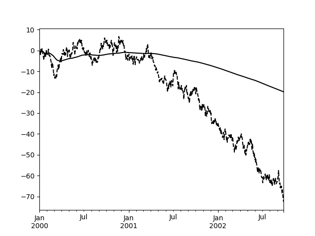
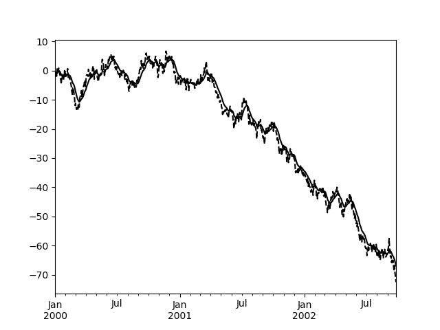
In [46]: s.plot(style='k--') Out[46]: <matplotlib.axes._subplots.AxesSubplot at 0x7faf83b476d8>
In [47]: r.mean().plot(style='k') Out[47]: <matplotlib.axes._subplots.AxesSubplot at 0x7faf83b476d8>

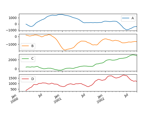
They can also be applied to DataFrame objects. This is really just syntactic sugar for applying the moving window operator to all of the DataFrame’s columns:
In [48]: df = pd.DataFrame(np.random.randn(1000, 4), ....: index=pd.date_range('1/1/2000', periods=1000), ....: columns=['A', 'B', 'C', 'D']) ....:
In [49]: df = df.cumsum()
In [50]: df.rolling(window=60).sum().plot(subplots=True) Out[50]: array([<matplotlib.axes._subplots.AxesSubplot object at 0x7faf8014a0b8>, <matplotlib.axes._subplots.AxesSubplot object at 0x7faf80171320>, <matplotlib.axes._subplots.AxesSubplot object at 0x7faf80118438>, <matplotlib.axes._subplots.AxesSubplot object at 0x7faf80142550>], dtype=object)
Method Summary
We provide a number of common statistical functions:
| Method | Description |
|---|---|
| count() | Number of non-null observations |
| sum() | Sum of values |
| mean() | Mean of values |
| median() | Arithmetic median of values |
| min() | Minimum |
| max() | Maximum |
| std() | Bessel-corrected sample standard deviation |
| var() | Unbiased variance |
| skew() | Sample skewness (3rd moment) |
| kurt() | Sample kurtosis (4th moment) |
| quantile() | Sample quantile (value at %) |
| apply() | Generic apply |
| cov() | Unbiased covariance (binary) |
| corr() | Correlation (binary) |
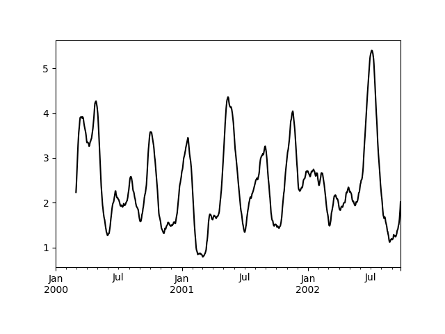
The apply() function takes an extra func argument and performs generic rolling computations. The func argument should be a single function that produces a single value from an ndarray input. Suppose we wanted to compute the mean absolute deviation on a rolling basis:
In [51]: def mad(x): ....: return np.fabs(x - x.mean()).mean() ....:
In [52]: s.rolling(window=60).apply(mad, raw=True).plot(style='k') Out[52]: <matplotlib.axes._subplots.AxesSubplot at 0x7faf800d3438>
Rolling Windows
Passing win_type to .rolling generates a generic rolling window computation, that is weighted according the win_type. The following methods are available:
| Method | Description |
|---|---|
| sum() | Sum of values |
| mean() | Mean of values |
The weights used in the window are specified by the win_type keyword. The list of recognized types are the scipy.signal window functions:
boxcartriangblackmanhammingbartlettparzenbohmanblackmanharrisnuttallbarthannkaiser(needs beta)gaussian(needs std)general_gaussian(needs power, width)slepian(needs width).
In [53]: ser = pd.Series(np.random.randn(10), ....: index=pd.date_range('1/1/2000', periods=10)) ....:
In [54]: ser.rolling(window=5, win_type='triang').mean() Out[54]: 2000-01-01 NaN 2000-01-02 NaN 2000-01-03 NaN 2000-01-04 NaN 2000-01-05 -1.037870 2000-01-06 -0.767705 2000-01-07 -0.383197 2000-01-08 -0.395513 2000-01-09 -0.558440 2000-01-10 -0.672416 Freq: D, dtype: float64
Note that the boxcar window is equivalent to mean().
In [55]: ser.rolling(window=5, win_type='boxcar').mean() Out[55]: 2000-01-01 NaN 2000-01-02 NaN 2000-01-03 NaN 2000-01-04 NaN 2000-01-05 -0.841164 2000-01-06 -0.779948 2000-01-07 -0.565487 2000-01-08 -0.502815 2000-01-09 -0.553755 2000-01-10 -0.472211 Freq: D, dtype: float64
In [56]: ser.rolling(window=5).mean() Out[56]: 2000-01-01 NaN 2000-01-02 NaN 2000-01-03 NaN 2000-01-04 NaN 2000-01-05 -0.841164 2000-01-06 -0.779948 2000-01-07 -0.565487 2000-01-08 -0.502815 2000-01-09 -0.553755 2000-01-10 -0.472211 Freq: D, dtype: float64
For some windowing functions, additional parameters must be specified:
In [57]: ser.rolling(window=5, win_type='gaussian').mean(std=0.1) Out[57]: 2000-01-01 NaN 2000-01-02 NaN 2000-01-03 NaN 2000-01-04 NaN 2000-01-05 -1.309989 2000-01-06 -1.153000 2000-01-07 0.606382 2000-01-08 -0.681101 2000-01-09 -0.289724 2000-01-10 -0.996632 Freq: D, dtype: float64
Note
For .sum() with a win_type, there is no normalization done to the weights for the window. Passing custom weights of [1, 1, 1] will yield a different result than passing weights of [2, 2, 2], for example. When passing awin_type instead of explicitly specifying the weights, the weights are already normalized so that the largest weight is 1.
In contrast, the nature of the .mean() calculation is such that the weights are normalized with respect to each other. Weights of [1, 1, 1] and [2, 2, 2] yield the same result.
Time-aware Rolling
New in version 0.19.0.
New in version 0.19.0 are the ability to pass an offset (or convertible) to a .rolling() method and have it produce variable sized windows based on the passed time window. For each time point, this includes all preceding values occurring within the indicated time delta.
This can be particularly useful for a non-regular time frequency index.
In [58]: dft = pd.DataFrame({'B': [0, 1, 2, np.nan, 4]}, ....: index=pd.date_range('20130101 09:00:00', ....: periods=5, ....: freq='s')) ....:
In [59]: dft Out[59]: B 2013-01-01 09:00:00 0.0 2013-01-01 09:00:01 1.0 2013-01-01 09:00:02 2.0 2013-01-01 09:00:03 NaN 2013-01-01 09:00:04 4.0
This is a regular frequency index. Using an integer window parameter works to roll along the window frequency.
In [60]: dft.rolling(2).sum() Out[60]: B 2013-01-01 09:00:00 NaN 2013-01-01 09:00:01 1.0 2013-01-01 09:00:02 3.0 2013-01-01 09:00:03 NaN 2013-01-01 09:00:04 NaN
In [61]: dft.rolling(2, min_periods=1).sum() Out[61]: B 2013-01-01 09:00:00 0.0 2013-01-01 09:00:01 1.0 2013-01-01 09:00:02 3.0 2013-01-01 09:00:03 2.0 2013-01-01 09:00:04 4.0
Specifying an offset allows a more intuitive specification of the rolling frequency.
In [62]: dft.rolling('2s').sum() Out[62]: B 2013-01-01 09:00:00 0.0 2013-01-01 09:00:01 1.0 2013-01-01 09:00:02 3.0 2013-01-01 09:00:03 2.0 2013-01-01 09:00:04 4.0
Using a non-regular, but still monotonic index, rolling with an integer window does not impart any special calculation.
In [63]: dft = pd.DataFrame({'B': [0, 1, 2, np.nan, 4]}, ....: index=pd.Index([pd.Timestamp('20130101 09:00:00'), ....: pd.Timestamp('20130101 09:00:02'), ....: pd.Timestamp('20130101 09:00:03'), ....: pd.Timestamp('20130101 09:00:05'), ....: pd.Timestamp('20130101 09:00:06')], ....: name='foo')) ....:
In [64]: dft
Out[64]:
B
foo
2013-01-01 09:00:00 0.0
2013-01-01 09:00:02 1.0
2013-01-01 09:00:03 2.0
2013-01-01 09:00:05 NaN
2013-01-01 09:00:06 4.0
In [65]: dft.rolling(2).sum()
Out[65]:
B
foo
2013-01-01 09:00:00 NaN
2013-01-01 09:00:02 1.0
2013-01-01 09:00:03 3.0
2013-01-01 09:00:05 NaN
2013-01-01 09:00:06 NaN
Using the time-specification generates variable windows for this sparse data.
In [66]: dft.rolling('2s').sum()
Out[66]:
B
foo
2013-01-01 09:00:00 0.0
2013-01-01 09:00:02 1.0
2013-01-01 09:00:03 3.0
2013-01-01 09:00:05 NaN
2013-01-01 09:00:06 4.0
Furthermore, we now allow an optional on parameter to specify a column (rather than the default of the index) in a DataFrame.
In [67]: dft = dft.reset_index()
In [68]: dft Out[68]: foo B 0 2013-01-01 09:00:00 0.0 1 2013-01-01 09:00:02 1.0 2 2013-01-01 09:00:03 2.0 3 2013-01-01 09:00:05 NaN 4 2013-01-01 09:00:06 4.0
In [69]: dft.rolling('2s', on='foo').sum() Out[69]: foo B 0 2013-01-01 09:00:00 0.0 1 2013-01-01 09:00:02 1.0 2 2013-01-01 09:00:03 3.0 3 2013-01-01 09:00:05 NaN 4 2013-01-01 09:00:06 4.0
Rolling Window Endpoints
New in version 0.20.0.
The inclusion of the interval endpoints in rolling window calculations can be specified with the closedparameter:
| closed | Description | Default for |
|---|---|---|
| right | close right endpoint | time-based windows |
| left | close left endpoint | |
| both | close both endpoints | fixed windows |
| neither | open endpoints |
For example, having the right endpoint open is useful in many problems that require that there is no contamination from present information back to past information. This allows the rolling window to compute statistics “up to that point in time”, but not including that point in time.
In [70]: df = pd.DataFrame({'x': 1}, ....: index=[pd.Timestamp('20130101 09:00:01'), ....: pd.Timestamp('20130101 09:00:02'), ....: pd.Timestamp('20130101 09:00:03'), ....: pd.Timestamp('20130101 09:00:04'), ....: pd.Timestamp('20130101 09:00:06')]) ....:
In [71]: df["right"] = df.rolling('2s', closed='right').x.sum() # default
In [72]: df["both"] = df.rolling('2s', closed='both').x.sum()
In [73]: df["left"] = df.rolling('2s', closed='left').x.sum()
In [74]: df["neither"] = df.rolling('2s', closed='neither').x.sum()
In [75]: df Out[75]: x right both left neither 2013-01-01 09:00:01 1 1.0 1.0 NaN NaN 2013-01-01 09:00:02 1 2.0 2.0 1.0 1.0 2013-01-01 09:00:03 1 2.0 3.0 2.0 1.0 2013-01-01 09:00:04 1 2.0 3.0 2.0 1.0 2013-01-01 09:00:06 1 1.0 2.0 1.0 NaN
Currently, this feature is only implemented for time-based windows. For fixed windows, the closed parameter cannot be set and the rolling window will always have both endpoints closed.
Time-aware Rolling vs. Resampling
Using .rolling() with a time-based index is quite similar to resampling. They both operate and perform reductive operations on time-indexed pandas objects.
When using .rolling() with an offset. The offset is a time-delta. Take a backwards-in-time looking window, and aggregate all of the values in that window (including the end-point, but not the start-point). This is the new value at that point in the result. These are variable sized windows in time-space for each point of the input. You will get a same sized result as the input.
When using .resample() with an offset. Construct a new index that is the frequency of the offset. For each frequency bin, aggregate points from the input within a backwards-in-time looking window that fall in that bin. The result of this aggregation is the output for that frequency point. The windows are fixed size in the frequency space. Your result will have the shape of a regular frequency between the min and the max of the original input object.
To summarize, .rolling() is a time-based window operation, while .resample() is a frequency-based window operation.
Centering Windows
By default the labels are set to the right edge of the window, but acenter keyword is available so the labels can be set at the center.
In [76]: ser.rolling(window=5).mean() Out[76]: 2000-01-01 NaN 2000-01-02 NaN 2000-01-03 NaN 2000-01-04 NaN 2000-01-05 -0.841164 2000-01-06 -0.779948 2000-01-07 -0.565487 2000-01-08 -0.502815 2000-01-09 -0.553755 2000-01-10 -0.472211 Freq: D, dtype: float64
In [77]: ser.rolling(window=5, center=True).mean() Out[77]: 2000-01-01 NaN 2000-01-02 NaN 2000-01-03 -0.841164 2000-01-04 -0.779948 2000-01-05 -0.565487 2000-01-06 -0.502815 2000-01-07 -0.553755 2000-01-08 -0.472211 2000-01-09 NaN 2000-01-10 NaN Freq: D, dtype: float64
Binary Window Functions
cov() and corr() can compute moving window statistics about two Series or any combination of DataFrame/Series orDataFrame/DataFrame. Here is the behavior in each case:
- two
Series: compute the statistic for the pairing. DataFrame/Series: compute the statistics for each column of the DataFrame with the passed Series, thus returning a DataFrame.DataFrame/DataFrame: by default compute the statistic for matching column names, returning a DataFrame. If the keyword argumentpairwise=Trueis passed then computes the statistic for each pair of columns, returning aMultiIndexed DataFramewhoseindexare the dates in question (see the next section).
For example:
In [78]: df = pd.DataFrame(np.random.randn(1000, 4), ....: index=pd.date_range('1/1/2000', periods=1000), ....: columns=['A', 'B', 'C', 'D']) ....:
In [79]: df = df.cumsum()
In [80]: df2 = df[:20]
In [81]: df2.rolling(window=5).corr(df2['B']) Out[81]: A B C D 2000-01-01 NaN NaN NaN NaN 2000-01-02 NaN NaN NaN NaN 2000-01-03 NaN NaN NaN NaN 2000-01-04 NaN NaN NaN NaN 2000-01-05 0.768775 1.0 -0.977990 0.800252 2000-01-06 0.744106 1.0 -0.967912 0.830021 2000-01-07 0.683257 1.0 -0.928969 0.384916 ... ... ... ... ... 2000-01-14 -0.392318 1.0 0.570240 -0.591056 2000-01-15 0.017217 1.0 0.649900 -0.896258 2000-01-16 0.691078 1.0 0.807450 -0.939302 2000-01-17 0.274506 1.0 0.582601 -0.902954 2000-01-18 0.330459 1.0 0.515707 -0.545268 2000-01-19 0.046756 1.0 -0.104334 -0.419799 2000-01-20 -0.328241 1.0 -0.650974 -0.777777
[20 rows x 4 columns]
Computing rolling pairwise covariances and correlations
Warning
Prior to version 0.20.0 if pairwise=True was passed, a Panel would be returned. This will now return a 2-level MultiIndexed DataFrame, see the whatsnew here.
In financial data analysis and other fields it’s common to compute covariance and correlation matrices for a collection of time series. Often one is also interested in moving-window covariance and correlation matrices. This can be done by passing the pairwise keyword argument, which in the case ofDataFrame inputs will yield a MultiIndexed DataFrame whose index are the dates in question. In the case of a single DataFrame argument the pairwise argument can even be omitted:
Note
Missing values are ignored and each entry is computed using the pairwise complete observations. Please see the covariance section for caveats associated with this method of calculating covariance and correlation matrices.
In [82]: covs = (df[['B', 'C', 'D']].rolling(window=50) ....: .cov(df[['A', 'B', 'C']], pairwise=True)) ....:
In [83]: covs.loc['2002-09-22':] Out[83]: B C D 2002-09-22 A 1.367467 8.676734 -8.047366 B 3.067315 0.865946 -1.052533 C 0.865946 7.739761 -4.943924 2002-09-23 A 0.910343 8.669065 -8.443062 B 2.625456 0.565152 -0.907654 C 0.565152 7.825521 -5.367526 2002-09-24 A 0.463332 8.514509 -8.776514 B 2.306695 0.267746 -0.732186 C 0.267746 7.771425 -5.696962 2002-09-25 A 0.467976 8.198236 -9.162599 B 2.307129 0.267287 -0.754080 C 0.267287 7.466559 -5.822650 2002-09-26 A 0.545781 7.899084 -9.326238 B 2.311058 0.322295 -0.844451 C 0.322295 7.038237 -5.684445
In [84]: correls = df.rolling(window=50).corr()
In [85]: correls.loc['2002-09-22':] Out[85]: A B C D 2002-09-22 A 1.000000 0.186397 0.744551 -0.769767 B 0.186397 1.000000 0.177725 -0.240802 C 0.744551 0.177725 1.000000 -0.712051 D -0.769767 -0.240802 -0.712051 1.000000 2002-09-23 A 1.000000 0.134723 0.743113 -0.758758 B 0.134723 1.000000 0.124683 -0.209934 C 0.743113 0.124683 1.000000 -0.719088 ... ... ... ... ... 2002-09-25 B 0.075157 1.000000 0.064399 -0.164179 C 0.731888 0.064399 1.000000 -0.704686 D -0.739160 -0.164179 -0.704686 1.000000 2002-09-26 A 1.000000 0.087756 0.727792 -0.736562 B 0.087756 1.000000 0.079913 -0.179477 C 0.727792 0.079913 1.000000 -0.692303 D -0.736562 -0.179477 -0.692303 1.000000
[20 rows x 4 columns]
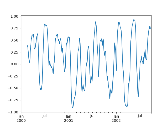
You can efficiently retrieve the time series of correlations between two columns by reshaping and indexing:
In [86]: correls.unstack(1)[('A', 'C')].plot() Out[86]: <matplotlib.axes._subplots.AxesSubplot at 0x7faf7b8455c0>
Aggregation
Once the Rolling, Expanding or EWM objects have been created, several methods are available to perform multiple computations on the data. These operations are similar to the aggregating API,groupby API, and resample API.
In [87]: dfa = pd.DataFrame(np.random.randn(1000, 3), ....: index=pd.date_range('1/1/2000', periods=1000), ....: columns=['A', 'B', 'C']) ....:
In [88]: r = dfa.rolling(window=60, min_periods=1)
In [89]: r Out[89]: Rolling [window=60,min_periods=1,center=False,axis=0]
We can aggregate by passing a function to the entire DataFrame, or select a Series (or multiple Series) via standard __getitem__.
In [90]: r.aggregate(np.sum) Out[90]: A B C 2000-01-01 -0.289838 -0.370545 -1.284206 2000-01-02 -0.216612 -1.675528 -1.169415 2000-01-03 1.154661 -1.634017 -1.566620 2000-01-04 2.969393 -4.003274 -1.816179 2000-01-05 4.690630 -4.682017 -2.717209 2000-01-06 3.880630 -4.447700 -1.078947 2000-01-07 4.001957 -2.884072 -3.116903 ... ... ... ... 2002-09-20 2.652493 -10.528875 9.867805 2002-09-21 0.844497 -9.280944 9.522649 2002-09-22 2.860036 -9.270337 6.415245 2002-09-23 3.510163 -8.151439 5.177219 2002-09-24 6.524983 -10.168078 5.792639 2002-09-25 6.409626 -9.956226 5.704050 2002-09-26 5.093787 -7.074515 6.905823
[1000 rows x 3 columns]
In [91]: r['A'].aggregate(np.sum)
Out[91]:
2000-01-01 -0.289838
2000-01-02 -0.216612
2000-01-03 1.154661
2000-01-04 2.969393
2000-01-05 4.690630
2000-01-06 3.880630
2000-01-07 4.001957
...
2002-09-20 2.652493
2002-09-21 0.844497
2002-09-22 2.860036
2002-09-23 3.510163
2002-09-24 6.524983
2002-09-25 6.409626
2002-09-26 5.093787
Freq: D, Name: A, Length: 1000, dtype: float64
In [92]: r[['A', 'B']].aggregate(np.sum) Out[92]: A B 2000-01-01 -0.289838 -0.370545 2000-01-02 -0.216612 -1.675528 2000-01-03 1.154661 -1.634017 2000-01-04 2.969393 -4.003274 2000-01-05 4.690630 -4.682017 2000-01-06 3.880630 -4.447700 2000-01-07 4.001957 -2.884072 ... ... ... 2002-09-20 2.652493 -10.528875 2002-09-21 0.844497 -9.280944 2002-09-22 2.860036 -9.270337 2002-09-23 3.510163 -8.151439 2002-09-24 6.524983 -10.168078 2002-09-25 6.409626 -9.956226 2002-09-26 5.093787 -7.074515
[1000 rows x 2 columns]
As you can see, the result of the aggregation will have the selected columns, or all columns if none are selected.
Applying multiple functions
With windowed Series you can also pass a list of functions to do aggregation with, outputting a DataFrame:
In [93]: r['A'].agg([np.sum, np.mean, np.std]) Out[93]: sum mean std 2000-01-01 -0.289838 -0.289838 NaN 2000-01-02 -0.216612 -0.108306 0.256725 2000-01-03 1.154661 0.384887 0.873311 2000-01-04 2.969393 0.742348 1.009734 2000-01-05 4.690630 0.938126 0.977914 2000-01-06 3.880630 0.646772 1.128883 2000-01-07 4.001957 0.571708 1.049487 ... ... ... ... 2002-09-20 2.652493 0.044208 1.164919 2002-09-21 0.844497 0.014075 1.148231 2002-09-22 2.860036 0.047667 1.132051 2002-09-23 3.510163 0.058503 1.134296 2002-09-24 6.524983 0.108750 1.144204 2002-09-25 6.409626 0.106827 1.142913 2002-09-26 5.093787 0.084896 1.151416
[1000 rows x 3 columns]
On a windowed DataFrame, you can pass a list of functions to apply to each column, which produces an aggregated result with a hierarchical index:
In [94]: r.agg([np.sum, np.mean])
Out[94]:
A B C
sum mean sum mean sum mean
2000-01-01 -0.289838 -0.289838 -0.370545 -0.370545 -1.284206 -1.284206
2000-01-02 -0.216612 -0.108306 -1.675528 -0.837764 -1.169415 -0.584708
2000-01-03 1.154661 0.384887 -1.634017 -0.544672 -1.566620 -0.522207
2000-01-04 2.969393 0.742348 -4.003274 -1.000819 -1.816179 -0.454045
2000-01-05 4.690630 0.938126 -4.682017 -0.936403 -2.717209 -0.543442
2000-01-06 3.880630 0.646772 -4.447700 -0.741283 -1.078947 -0.179825
2000-01-07 4.001957 0.571708 -2.884072 -0.412010 -3.116903 -0.445272
... ... ... ... ... ... ...
2002-09-20 2.652493 0.044208 -10.528875 -0.175481 9.867805 0.164463
2002-09-21 0.844497 0.014075 -9.280944 -0.154682 9.522649 0.158711
2002-09-22 2.860036 0.047667 -9.270337 -0.154506 6.415245 0.106921
2002-09-23 3.510163 0.058503 -8.151439 -0.135857 5.177219 0.086287
2002-09-24 6.524983 0.108750 -10.168078 -0.169468 5.792639 0.096544
2002-09-25 6.409626 0.106827 -9.956226 -0.165937 5.704050 0.095068
2002-09-26 5.093787 0.084896 -7.074515 -0.117909 6.905823 0.115097
[1000 rows x 6 columns]
Passing a dict of functions has different behavior by default, see the next section.
Applying different functions to DataFrame columns
By passing a dict to aggregate you can apply a different aggregation to the columns of a DataFrame:
In [95]: r.agg({'A': np.sum, 'B': lambda x: np.std(x, ddof=1)}) Out[95]: A B 2000-01-01 -0.289838 NaN 2000-01-02 -0.216612 0.660747 2000-01-03 1.154661 0.689929 2000-01-04 2.969393 1.072199 2000-01-05 4.690630 0.939657 2000-01-06 3.880630 0.966848 2000-01-07 4.001957 1.240137 ... ... ... 2002-09-20 2.652493 1.114814 2002-09-21 0.844497 1.113220 2002-09-22 2.860036 1.113208 2002-09-23 3.510163 1.132381 2002-09-24 6.524983 1.080963 2002-09-25 6.409626 1.082911 2002-09-26 5.093787 1.136199
[1000 rows x 2 columns]
The function names can also be strings. In order for a string to be valid it must be implemented on the windowed object
In [96]: r.agg({'A': 'sum', 'B': 'std'}) Out[96]: A B 2000-01-01 -0.289838 NaN 2000-01-02 -0.216612 0.660747 2000-01-03 1.154661 0.689929 2000-01-04 2.969393 1.072199 2000-01-05 4.690630 0.939657 2000-01-06 3.880630 0.966848 2000-01-07 4.001957 1.240137 ... ... ... 2002-09-20 2.652493 1.114814 2002-09-21 0.844497 1.113220 2002-09-22 2.860036 1.113208 2002-09-23 3.510163 1.132381 2002-09-24 6.524983 1.080963 2002-09-25 6.409626 1.082911 2002-09-26 5.093787 1.136199
[1000 rows x 2 columns]
Furthermore you can pass a nested dict to indicate different aggregations on different columns.
In [97]: r.agg({'A': ['sum', 'std'], 'B': ['mean', 'std']})
Out[97]:
A B
sum std mean std
2000-01-01 -0.289838 NaN -0.370545 NaN
2000-01-02 -0.216612 0.256725 -0.837764 0.660747
2000-01-03 1.154661 0.873311 -0.544672 0.689929
2000-01-04 2.969393 1.009734 -1.000819 1.072199
2000-01-05 4.690630 0.977914 -0.936403 0.939657
2000-01-06 3.880630 1.128883 -0.741283 0.966848
2000-01-07 4.001957 1.049487 -0.412010 1.240137
... ... ... ... ...
2002-09-20 2.652493 1.164919 -0.175481 1.114814
2002-09-21 0.844497 1.148231 -0.154682 1.113220
2002-09-22 2.860036 1.132051 -0.154506 1.113208
2002-09-23 3.510163 1.134296 -0.135857 1.132381
2002-09-24 6.524983 1.144204 -0.169468 1.080963
2002-09-25 6.409626 1.142913 -0.165937 1.082911
2002-09-26 5.093787 1.151416 -0.117909 1.136199
[1000 rows x 4 columns]
Expanding Windows
A common alternative to rolling statistics is to use an expanding window, which yields the value of the statistic with all the data available up to that point in time.
These follow a similar interface to .rolling, with the .expanding method returning an Expanding object.
As these calculations are a special case of rolling statistics, they are implemented in pandas such that the following two calls are equivalent:
In [98]: df.rolling(window=len(df), min_periods=1).mean()[:5] Out[98]: A B C D 2000-01-01 0.314226 -0.001675 0.071823 0.892566 2000-01-02 0.654522 -0.171495 0.179278 0.853361 2000-01-03 0.708733 -0.064489 -0.238271 1.371111 2000-01-04 0.987613 0.163472 -0.919693 1.566485 2000-01-05 1.426971 0.288267 -1.358877 1.808650
In [99]: df.expanding(min_periods=1).mean()[:5] Out[99]: A B C D 2000-01-01 0.314226 -0.001675 0.071823 0.892566 2000-01-02 0.654522 -0.171495 0.179278 0.853361 2000-01-03 0.708733 -0.064489 -0.238271 1.371111 2000-01-04 0.987613 0.163472 -0.919693 1.566485 2000-01-05 1.426971 0.288267 -1.358877 1.808650
These have a similar set of methods to .rolling methods.
Method Summary
| Function | Description |
|---|---|
| count() | Number of non-null observations |
| sum() | Sum of values |
| mean() | Mean of values |
| median() | Arithmetic median of values |
| min() | Minimum |
| max() | Maximum |
| std() | Unbiased standard deviation |
| var() | Unbiased variance |
| skew() | Unbiased skewness (3rd moment) |
| kurt() | Unbiased kurtosis (4th moment) |
| quantile() | Sample quantile (value at %) |
| apply() | Generic apply |
| cov() | Unbiased covariance (binary) |
| corr() | Correlation (binary) |
Aside from not having a window parameter, these functions have the same interfaces as their .rolling counterparts. Like above, the parameters they all accept are:
min_periods: threshold of non-null data points to require. Defaults to minimum needed to compute statistic. NoNaNswill be output oncemin_periodsnon-null data points have been seen.center: boolean, whether to set the labels at the center (default is False).
Note
The output of the .rolling and .expanding methods do not return aNaN if there are at least min_periods non-null values in the current window. For example:
In [100]: sn = pd.Series([1, 2, np.nan, 3, np.nan, 4])
In [101]: sn Out[101]: 0 1.0 1 2.0 2 NaN 3 3.0 4 NaN 5 4.0 dtype: float64
In [102]: sn.rolling(2).max() Out[102]: 0 NaN 1 2.0 2 NaN 3 NaN 4 NaN 5 NaN dtype: float64
In [103]: sn.rolling(2, min_periods=1).max() Out[103]: 0 1.0 1 2.0 2 2.0 3 3.0 4 3.0 5 4.0 dtype: float64
In case of expanding functions, this differs from cumsum(),cumprod(), cummax(), and cummin(), which return NaN in the output wherever a NaN is encountered in the input. In order to match the output of cumsumwith expanding, use fillna():
In [104]: sn.expanding().sum() Out[104]: 0 1.0 1 3.0 2 3.0 3 6.0 4 6.0 5 10.0 dtype: float64
In [105]: sn.cumsum() Out[105]: 0 1.0 1 3.0 2 NaN 3 6.0 4 NaN 5 10.0 dtype: float64
In [106]: sn.cumsum().fillna(method='ffill') Out[106]: 0 1.0 1 3.0 2 3.0 3 6.0 4 6.0 5 10.0 dtype: float64
An expanding window statistic will be more stable (and less responsive) than its rolling window counterpart as the increasing window size decreases the relative impact of an individual data point. As an example, here is themean() output for the previous time series dataset:
In [107]: s.plot(style='k--') Out[107]: <matplotlib.axes._subplots.AxesSubplot at 0x7faf8a10d630>
In [108]: s.expanding().mean().plot(style='k') Out[108]: <matplotlib.axes._subplots.AxesSubplot at 0x7faf8a10d630>
Exponentially Weighted Windows
A related set of functions are exponentially weighted versions of several of the above statistics. A similar interface to .rolling and .expanding is accessed through the .ewm method to receive an EWM object. A number of expanding EW (exponentially weighted) methods are provided:
| Function | Description |
|---|---|
| mean() | EW moving average |
| var() | EW moving variance |
| std() | EW moving standard deviation |
| corr() | EW moving correlation |
| cov() | EW moving covariance |
In general, a weighted moving average is calculated as
\[y_t = \frac{\sum_{i=0}^t w_i x_{t-i}}{\sum_{i=0}^t w_i},\]
where \(x_t\) is the input, \(y_t\) is the result and the \(w_i\)are the weights.
The EW functions support two variants of exponential weights. The default, adjust=True, uses the weights \(w_i = (1 - \alpha)^i\)which gives
\[y_t = \frac{x_t + (1 - \alpha)x_{t-1} + (1 - \alpha)^2 x_{t-2} + ... + (1 - \alpha)^t x_{0}}{1 + (1 - \alpha) + (1 - \alpha)^2 + ... + (1 - \alpha)^t}\]
When adjust=False is specified, moving averages are calculated as
\[\begin{split}y_0 &= x_0 \\ y_t &= (1 - \alpha) y_{t-1} + \alpha x_t,\end{split}\]
which is equivalent to using weights
\[\begin{split}w_i = \begin{cases} \alpha (1 - \alpha)^i & \text{if } i < t \\ (1 - \alpha)^i & \text{if } i = t. \end{cases}\end{split}\]
Note
These equations are sometimes written in terms of \(\alpha' = 1 - \alpha\), e.g.
\[y_t = \alpha' y_{t-1} + (1 - \alpha') x_t.\]
The difference between the above two variants arises because we are dealing with series which have finite history. Consider a series of infinite history:
\[y_t = \frac{x_t + (1 - \alpha)x_{t-1} + (1 - \alpha)^2 x_{t-2} + ...} {1 + (1 - \alpha) + (1 - \alpha)^2 + ...}\]
Noting that the denominator is a geometric series with initial term equal to 1 and a ratio of \(1 - \alpha\) we have
\[\begin{split}y_t &= \frac{x_t + (1 - \alpha)x_{t-1} + (1 - \alpha)^2 x_{t-2} + ...} {\frac{1}{1 - (1 - \alpha)}}\\ &= [x_t + (1 - \alpha)x_{t-1} + (1 - \alpha)^2 x_{t-2} + ...] \alpha \\ &= \alpha x_t + [(1-\alpha)x_{t-1} + (1 - \alpha)^2 x_{t-2} + ...]\alpha \\ &= \alpha x_t + (1 - \alpha)[x_{t-1} + (1 - \alpha) x_{t-2} + ...]\alpha\\ &= \alpha x_t + (1 - \alpha) y_{t-1}\end{split}\]
which shows the equivalence of the above two variants for infinite series. When adjust=True we have \(y_0 = x_0\) and from the last representation above we have \(y_t = \alpha x_t + (1 - \alpha) y_{t-1}\), therefore there is an assumption that \(x_0\) is not an ordinary value but rather an exponentially weighted moment of the infinite series up to that point.
One must have \(0 < \alpha \leq 1\), and while since version 0.18.0 it has been possible to pass \(\alpha\) directly, it’s often easier to think about either the span, center of mass (com) or half-lifeof an EW moment:
\[\begin{split}\alpha = \begin{cases} \frac{2}{s + 1}, & \text{for span}\ s \geq 1\\ \frac{1}{1 + c}, & \text{for center of mass}\ c \geq 0\\ 1 - \exp^{\frac{\log 0.5}{h}}, & \text{for half-life}\ h > 0 \end{cases}\end{split}\]
One must specify precisely one of span, center of mass, half-lifeand alpha to the EW functions:
- Span corresponds to what is commonly called an “N-day EW moving average”.
- Center of mass has a more physical interpretation and can be thought of in terms of span: \(c = (s - 1) / 2\).
- Half-life is the period of time for the exponential weight to reduce to one half.
- Alpha specifies the smoothing factor directly.
Here is an example for a univariate time series:
In [109]: s.plot(style='k--') Out[109]: <matplotlib.axes._subplots.AxesSubplot at 0x7faf7b656390>
In [110]: s.ewm(span=20).mean().plot(style='k') Out[110]: <matplotlib.axes._subplots.AxesSubplot at 0x7faf7b656390>
EWM has a min_periods argument, which has the same meaning it does for all the .expanding and .rolling methods: no output values will be set until at least min_periods non-null values are encountered in the (expanding) window.
EWM also has an ignore_na argument, which determines how intermediate null values affect the calculation of the weights. When ignore_na=False (the default), weights are calculated based on absolute positions, so that intermediate null values affect the result. When ignore_na=True, weights are calculated by ignoring intermediate null values. For example, assuming adjust=True, if ignore_na=False, the weighted average of 3, NaN, 5 would be calculated as
\[\frac{(1-\alpha)^2 \cdot 3 + 1 \cdot 5}{(1-\alpha)^2 + 1}.\]
Whereas if ignore_na=True, the weighted average would be calculated as
\[\frac{(1-\alpha) \cdot 3 + 1 \cdot 5}{(1-\alpha) + 1}.\]
The var(), std(), and cov() functions have a bias argument, specifying whether the result should contain biased or unbiased statistics. For example, if bias=True, ewmvar(x) is calculated asewmvar(x) = ewma(x**2) - ewma(x)**2; whereas if bias=False (the default), the biased variance statistics are scaled by debiasing factors
\[\frac{\left(\sum_{i=0}^t w_i\right)^2}{\left(\sum_{i=0}^t w_i\right)^2 - \sum_{i=0}^t w_i^2}.\]
(For \(w_i = 1\), this reduces to the usual \(N / (N - 1)\) factor, with \(N = t + 1\).) See Weighted Sample Varianceon Wikipedia for further details.