DecisionBoundaryDisplay (original) (raw)
class sklearn.inspection.DecisionBoundaryDisplay(*, xx0, xx1, response, xlabel=None, ylabel=None)[source]#
Decisions boundary visualization.
It is recommended to usefrom_estimatorto create a DecisionBoundaryDisplay. All parameters are stored as attributes.
Read more in the User Guide.
Added in version 1.1.
Parameters:
xx0ndarray of shape (grid_resolution, grid_resolution)
First output of meshgrid.
xx1ndarray of shape (grid_resolution, grid_resolution)
Second output of meshgrid.
responsendarray of shape (grid_resolution, grid_resolution)
Values of the response function.
xlabelstr, default=None
Default label to place on x axis.
ylabelstr, default=None
Default label to place on y axis.
Attributes:
**surface_**matplotlib QuadContourSet or QuadMesh
If plot_method is ‘contour’ or ‘contourf’, surface_ is aQuadContourSet. Ifplot_method is ‘pcolormesh’, surface_ is aQuadMesh.
**ax_**matplotlib Axes
Axes with decision boundary.
**figure_**matplotlib Figure
Figure containing the decision boundary.
See also
DecisionBoundaryDisplay.from_estimator
Plot decision boundary given an estimator.
Examples
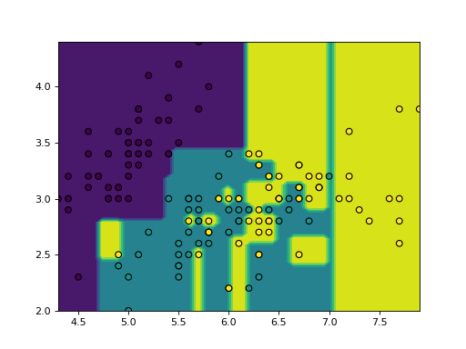
import matplotlib.pyplot as plt import numpy as np from sklearn.datasets import load_iris from sklearn.inspection import DecisionBoundaryDisplay from sklearn.tree import DecisionTreeClassifier iris = load_iris() feature_1, feature_2 = np.meshgrid( ... np.linspace(iris.data[:, 0].min(), iris.data[:, 0].max()), ... np.linspace(iris.data[:, 1].min(), iris.data[:, 1].max()) ... ) grid = np.vstack([feature_1.ravel(), feature_2.ravel()]).T tree = DecisionTreeClassifier().fit(iris.data[:, :2], iris.target) y_pred = np.reshape(tree.predict(grid), feature_1.shape) display = DecisionBoundaryDisplay( ... xx0=feature_1, xx1=feature_2, response=y_pred ... ) display.plot() <...> display.ax_.scatter( ... iris.data[:, 0], iris.data[:, 1], c=iris.target, edgecolor="black" ... ) <...> plt.show()

classmethod from_estimator(estimator, X, *, grid_resolution=100, eps=1.0, plot_method='contourf', response_method='auto', class_of_interest=None, xlabel=None, ylabel=None, ax=None, **kwargs)[source]#
Plot decision boundary given an estimator.
Read more in the User Guide.
Parameters:
estimatorobject
Trained estimator used to plot the decision boundary.
X{array-like, sparse matrix, dataframe} of shape (n_samples, 2)
Input data that should be only 2-dimensional.
grid_resolutionint, default=100
Number of grid points to use for plotting decision boundary. Higher values will make the plot look nicer but be slower to render.
epsfloat, default=1.0
Extends the minimum and maximum values of X for evaluating the response function.
plot_method{‘contourf’, ‘contour’, ‘pcolormesh’}, default=’contourf’
Plotting method to call when plotting the response. Please refer to the following matplotlib documentation for details:contourf,contour,pcolormesh.
response_method{‘auto’, ‘predict_proba’, ‘decision_function’, ‘predict’}, default=’auto’
Specifies whether to use predict_proba,decision_function, predict as the target response. If set to ‘auto’, the response method is tried in the following order:decision_function, predict_proba, predict. For multiclass problems, predict is selected whenresponse_method="auto".
class_of_interestint, float, bool or str, default=None
The class considered when plotting the decision. If None,estimator.classes_[1] is considered as the positive class for binary classifiers. Must have an explicit value for multiclass classifiers when response_method is ‘predict_proba’ or ‘decision_function’.
Added in version 1.4.
xlabelstr, default=None
The label used for the x-axis. If None, an attempt is made to extract a label from X if it is a dataframe, otherwise an empty string is used.
ylabelstr, default=None
The label used for the y-axis. If None, an attempt is made to extract a label from X if it is a dataframe, otherwise an empty string is used.
axMatplotlib axes, default=None
Axes object to plot on. If None, a new figure and axes is created.
**kwargsdict
Additional keyword arguments to be passed to theplot_method.
Returns:
displayDecisionBoundaryDisplay
Object that stores the result.
Examples
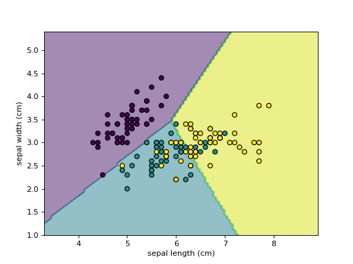
import matplotlib.pyplot as plt from sklearn.datasets import load_iris from sklearn.linear_model import LogisticRegression from sklearn.inspection import DecisionBoundaryDisplay iris = load_iris() X = iris.data[:, :2] classifier = LogisticRegression().fit(X, iris.target) disp = DecisionBoundaryDisplay.from_estimator( ... classifier, X, response_method="predict", ... xlabel=iris.feature_names[0], ylabel=iris.feature_names[1], ... alpha=0.5, ... ) disp.ax_.scatter(X[:, 0], X[:, 1], c=iris.target, edgecolor="k") <...> plt.show()

plot(plot_method='contourf', ax=None, xlabel=None, ylabel=None, **kwargs)[source]#
Plot visualization.
Parameters:
plot_method{‘contourf’, ‘contour’, ‘pcolormesh’}, default=’contourf’
Plotting method to call when plotting the response. Please refer to the following matplotlib documentation for details:contourf,contour,pcolormesh.
axMatplotlib axes, default=None
Axes object to plot on. If None, a new figure and axes is created.
xlabelstr, default=None
Overwrite the x-axis label.
ylabelstr, default=None
Overwrite the y-axis label.
**kwargsdict
Additional keyword arguments to be passed to the plot_method.
Returns:
display: DecisionBoundaryDisplay
Object that stores computed values.