Investigate Audio Classifications Using Deep Learning Interpretability Techniques - MATLAB & Simulink (original) (raw)

This example shows how to use interpretability techniques to investigate the predictions of a deep neural network trained to classify audio data.

Deep learning networks are often described as "black boxes" because why a network makes a certain decision is not always obvious. You can use interpretability techniques to translate network behavior into output that a person can interpret. This interpretable output can then answer questions about the predictions of a network. This example uses interpretability techniques that explain network predictions using visual representations of what a network is “looking” at. You can then use these visual representations to see which parts of the input images the network is using to make decisions.

This example uses transfer learning to retrain VGGish, a pretrained convolutional neural network, to classify a new set of audio signals.

Load Data

Download and unzip the environmental sound classification data set. This data set consists of recordings labeled as one of 10 different audio sound classes (ESC-10). Download the ESC-10.zip zip file from the MathWorks website, then unzip the file.

rng("default") zipFile = matlab.internal.examples.downloadSupportFile("audio","ESC-10.zip");

filepath = fileparts(zipFile); dataFolder = fullfile(filepath,"ESC-10"); unzip(zipFile,dataFolder)

Create an audioDatastore object to manage the data and split it into training and validation sets. Use countEachLabel to display the distribution of sound classes and the number of unique labels.

ads = audioDatastore(dataFolder,IncludeSubfolders=true,LabelSource="foldernames"); labelTable = countEachLabel(ads)

labelTable=10×2 table Label Count ______________ _____

chainsaw           40  
clock_tick         40  
crackling_fire     40  
crying_baby        40  
dog                40  
helicopter         40  
rain               40  
rooster            38  
sea_waves          40  
sneezing           40

Determine the total number of classes.

classes = labelTable.Label; numClasses = size(labelTable,1);

Use splitEachLabel to split the data set into training and validation sets. Use 80% of the data for training and 20% for validation.

[adsTrain,adsValidation] = splitEachLabel(ads,0.8,0.2);

The VGGish pretrained network requires preprocessing of the audio signals into log mel spectrograms. The supporting function helperAudioPreprocess, defined at the end of this example, takes as input an audioDatastore object and the overlap percentage between log mel spectrograms and returns matrices of predictors and responses suitable for input to the VGGish network. Each audio file is split into several segments to feed into the VGGish network.

overlapPercentage = 75;

[trainFeatures,trainLabels] = helperAudioPreprocess(adsTrain,overlapPercentage); [validationFeatures,validationLabels,segmentsPerFile] = helperAudioPreprocess(adsValidation,overlapPercentage);

Visualize Data

View a random sample of the data.

numImages = 9; idxSubset = randi(numel(trainLabels),1,numImages);

viewingAngle = [90 -90];

figure tiledlayout("flow",TileSpacing="compact"); for i = 1:numImages img = trainFeatures(:,:,:,idxSubset(i)); label = trainLabels(idxSubset(i)); nexttile surf(img,EdgeColor="none") view(viewingAngle) title("Class: " + string(label),interpreter="none") end colormap parula

Build Network

This example uses transfer learning to retrain VGGish, a pretrained convolutional neural network, to classify a new set of audio signals.

Download VGGish Network

Download and unzip the Audio Toolbox™ model for VGGish.

Type vggish in the Command Window. If the Audio Toolbox model for VGGish is not installed, then the function provides a link to the location of the network weights. To download the model, click the link. Unzip the file to a location on the MATLAB path.

Load the VGGish model and convert it to a layerGraph object.

pretrainedNetwork = vggish; lgraph = layerGraph(pretrainedNetwork.Layers);

Prepare Network for Transfer Learning

Prepare the network for transfer learning by replacing the final layers with new layers suitable for the new data. You can adapt VGGish for the new data programmatically or interactively using Deep Network Designer. For an example showing how to use Deep Network Designer to perform transfer learning with an audio classification network, see Adapt Pretrained Audio Network for New Data Using Deep Network Designer.

Use removeLayers to remove the final regression output layer from the graph. After you remove the regression layer, the new final layer of the graph is a ReLU layer named EmbeddingBatch.

lgraph = removeLayers(lgraph,"regressionoutput"); lgraph.Layers(end)

ans = ReLULayer with properties:

Name: 'EmbeddingBatch'

Use addLayers to add a fullyConnectedLayer, a softmaxLayer, and a classificationLayer to the layer graph.

lgraph = addLayers(lgraph,fullyConnectedLayer(numClasses,Name="FCFinal")); lgraph = addLayers(lgraph,softmaxLayer(Name="softmax")); lgraph = addLayers(lgraph,classificationLayer(Name="classOut"));

Use connectLayers to append the fully connected, softmax, and classification layers to the layer graph.

lgraph = connectLayers(lgraph,"EmbeddingBatch","FCFinal"); lgraph = connectLayers(lgraph,"FCFinal","softmax"); lgraph = connectLayers(lgraph,"softmax","classOut");

Specify Training Options

To define the training options, use the trainingOptions function. Set the solver to "adam" and train for five epochs with a mini-batch size of 128. Specify an initial learning rate of 0.001 and drop the learning rate after two epochs by multiplying by a factor of 0.5. Monitor the network accuracy during training by specifying validation data and the validation frequency.

miniBatchSize = 128; options = trainingOptions("adam", ... MaxEpochs=5, ... MiniBatchSize=miniBatchSize, ... InitialLearnRate = 0.001, ... LearnRateSchedule="piecewise", ... LearnRateDropPeriod=2, ... LearnRateDropFactor=0.5, ... ValidationData={validationFeatures,validationLabels}, ... ValidationFrequency=50, ... Shuffle="every-epoch");

Train Network

To train the network, use the trainNetwork function. By default, trainNetwork uses a GPU if one is available. Otherwise, it uses a CPU. Training on a GPU requires Parallel Computing Toolbox™ and a supported GPU device. For information on supported devices, see GPU Computing Requirements (Parallel Computing Toolbox). You can also specify the execution environment by using the ExecutionEnvironment name-value argument of trainingOptions.

[net,netInfo] = trainNetwork(trainFeatures,trainLabels,lgraph,options);

Training on single GPU. |======================================================================================================================| | Epoch | Iteration | Time Elapsed | Mini-batch | Validation | Mini-batch | Validation | Base Learning | | | | (hh:mm:ss) | Accuracy | Accuracy | Loss | Loss | Rate | |======================================================================================================================| | 1 | 1 | 00:00:17 | 3.91% | 20.07% | 2.4103 | 2.1531 | 0.0010 | | 2 | 50 | 00:00:22 | 96.88% | 82.57% | 0.1491 | 0.7013 | 0.0010 | | 3 | 100 | 00:00:27 | 92.19% | 83.75% | 0.1730 | 0.7196 | 0.0005 | | 4 | 150 | 00:00:32 | 94.53% | 85.15% | 0.1654 | 0.8350 | 0.0005 | | 5 | 200 | 00:00:37 | 96.09% | 85.96% | 0.1747 | 0.8034 | 0.0003 | | 5 | 210 | 00:00:38 | 93.75% | 86.03% | 0.1643 | 0.7835 | 0.0003 | |======================================================================================================================| Training finished: Max epochs completed.

Test Network

Classify the validation mel spectrograms using the trained network.

[validationPredictions,validationScores] = classify(net,validationFeatures);

Each audio file produces multiple mel spectrograms. Combine the predictions for each audio file in the validation set using a majority-rule decision and calculate the classification accuracy.

idx = 1; validationPredictionsPerFile = categorical; for ii = 1:numel(adsValidation.Files) validationPredictionsPerFile(ii,1) = mode(validationPredictions(idx:idx+segmentsPerFile(ii)-1)); idx = idx + segmentsPerFile(ii); end

accuracy = mean(validationPredictionsPerFile==adsValidation.Labels)*100

Use confusionchart to evaluate the performance of the network on the validation set.

figure(Units="normalized",Position=[0.2 0.2 0.5 0.5]); cm = confusionchart(adsValidation.Labels,validationPredictionsPerFile); cm.Title = sprintf("Confusion Matrix for Validation Data \nAccuracy = %0.2f %%",accuracy); cm.ColumnSummary = "column-normalized"; cm.RowSummary = "row-normalized";

Visualize Predictions

View a random sample of the input data with the true and predicted class labels.

The _x_-axis represents time, the _y_-axis represents frequency, and the colormap represents decibels. For several of the classes, you can see interpretable features. For example, the spectrogram for the clock_tick class shows a repeating pattern through time representing the ticking of a clock. The first spectrogram from the helicopter class has the constant, loud, low-frequency sound of the helicopter engine and a repeating high-frequency sound representing the spinning of the helicopter blades.

As the network is a convolutional neural network with image input, the network might use these features when making classification decisions. You can investigate this hypothesis using deep learning interpretability techniques.

Investigate Predictions

Investigate the predictions of the validation mel spectrograms. For each input, generate the Grad-CAM (gradCAM), LIME (imageLIME), and occlusion sensitivity (occlusionSensitivity) maps for the predicted classes. These methods take an input image and a class label and produce a map indicating the regions of the image that are important to the score for the specified class. Each visualization method has a specific approach that determines the output it produces.

Grad-CAM — Use the gradient of the classification score with respect to the convolutional features determined by the network to understand which parts of the image are most important for classification. The places where the gradient is large are the places where the final score depends most on the data.
LIME — Approximate the classification behavior of a deep learning network using a simpler, more interpretable model, such as a linear model or a regression tree. The simple model determines the importance of features of the input data as a proxy for the importance of the features to the deep learning network.
Occlusion sensitivity — Perturb small areas of the input by replacing them with an occluding mask, typically a gray square. As the mask moves across the image, the technique measures the change in probability score for a given class.

Comparing the results of different interpretability techniques is important for verifying the conclusions you make. For more information about these techniques, see Deep Learning Visualization Methods.

Using the supporting function helperPlotMaps, defined at the end of this example, plot the input log mel spectrogram and the three interpretability maps for a selection of images and their predicted classes.

viewingAngle = [90 -90]; imgIdx = [250 500 750]; numImages = length(imgIdx);

figure t2 = tiledlayout(numImages,4,TileSpacing="compact"); for i = 1:numImages

img = validationFeatures(:,:,:,imgIdx(i));
YPred = validationPredictions(imgIdx(i));
YTrue = validationLabels(imgIdx(i));

mapClass = YPred;

mapGradCAM = gradCAM(net,img,mapClass, ...
    OutputUpsampling="nearest");

mapLIME = imageLIME(net,img,mapClass, ...
    OutputUpsampling="nearest", ...
    Segmentation="grid");

mapOcclusion = occlusionSensitivity(net,img,mapClass, ...
    OutputUpsampling="nearest");

maps = {mapGradCAM,mapLIME,mapOcclusion};
mapNames = ["Grad-CAM","LIME","Occlusion Sensitivity"];

helperPlotMaps(img,YPred,YTrue,maps,mapNames,viewingAngle,mapClass)

end

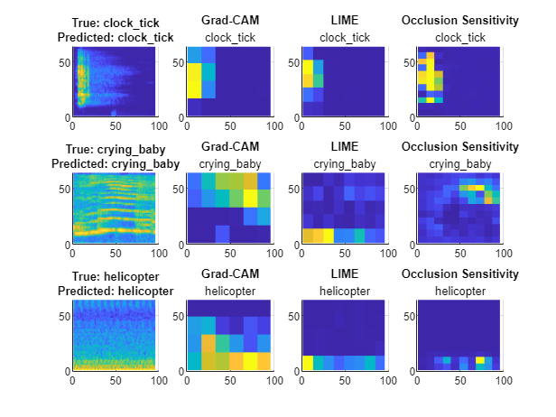
The interpretability mappings highlight regions of interest for the predicted class label of each spectrogram.

For the clock_tick class, all three methods focus on the same area of interest. The network uses the region corresponding to the ticking sound to make its prediction.
For the helicopter class, all the three methods focus on the same region at the bottom of the spectrogram.
For the crying_baby class, the three methods highlight different areas of the spectrogram, possibly because this spectrogram contains many small features. Methods like Grad-CAM, which produce lower resolution maps, might have difficulty picking out meaningful features. This example highlights the limits of using interpretability methods to understand individual network predictions.

As the results of training have an element of randomness, if you run this example again, you might see different results. Additionally, to produce interpretable output for different images, you might need to adjust the map parameters for the occlusion sensitivity and LIME maps. Grad-CAM does not require parameter tuning, but it can produce lower resolution maps than the other two methods.

Investigate Predictions for Specific Class

Investigate the interpretability maps for spectrograms from a particular class.

Find the spectrograms corresponding to the helicopter class.

classToInvestigate = "helicopter"; idxClass = find(classes == classToInvestigate); idxSubset = validationLabels==classes(idxClass);

subsetLabels = validationLabels(idxSubset); subsetImages = validationFeatures(:,:,:,idxSubset); subsetPredictions = validationPredictions(idxSubset);

imgIdx = [25 50 100]; numImages = length(imgIdx);

Generate and plot the interpretability maps using the input spectrograms and the predicted class labels.

viewingAngle = [90 -90];

figure t3 = tiledlayout(numImages,4,"TileSpacing","compact"); for i = 1:numImages

img = subsetImages(:,:,:,imgIdx(i));
YPred = subsetPredictions(imgIdx(i));
YTrue = subsetLabels(imgIdx(i));

mapClass = YPred;

mapGradCAM = gradCAM(net,img,mapClass, ...
    OutputUpsampling="nearest");

mapLIME = imageLIME(net,img,mapClass, ...
    OutputUpsampling="nearest", ...
    Segmentation="grid");

mapOcclusion = occlusionSensitivity(net,img,mapClass, ...
    OutputUpsampling="nearest");

maps = {mapGradCAM,mapLIME,mapOcclusion};
mapNames = ["Grad-CAM","LIME","Occlusion Sensitivity"];

helperPlotMaps(img,YPred,YTrue,maps,mapNames,viewingAngle,mapClass)

end

The maps for each image show that the network is focusing on the area of high intensity and low frequency. The result is surprising as you might expect the network to also be interested in the high-frequency noise that repeats through time. Spotting patterns like this is important for understanding the features a network is using to make predictions.

Investigate Misclassifications

Use the interpretability maps to investigate misclassifications.

Investigate a spectrogram with the true class chainsaw but the predicted class helicopter.

Generate and plot the maps for both the true class (chainsaw) and the predicted class (helicopter).

figure t4 = tiledlayout(2,4,"TileSpacing","compact"); img = validationFeatures(:,:,:,idxToInvestigate);

for mapClass = [YPred, YTrue]

mapGradCAM = gradCAM(net,img,mapClass, ...
    OutputUpsampling="nearest");

mapLIME = imageLIME(net,img,mapClass, ...
    OutputUpsampling="nearest", ...
    Segmentation="grid");

mapOcclusion = occlusionSensitivity(net,img,mapClass, ...
    OutputUpsampling="nearest");

maps = {mapGradCAM,mapLIME,mapOcclusion};
mapNames = ["Grad-CAM","LIME","Occlusion Sensitivity"];

helperPlotMaps(img,YPred,YTrue,maps,mapNames,viewingAngle,mapClass)

end

The network focuses on the area of low frequency for the helicopter class. The result matches the interpretability maps generated for the helicopter class. Visual inspection is important for investigating what parts of an input the network is using to make its classification decisions.

Supporting Functions

`helperPlotMaps`

The supporting function helperPlotMap generates a plot of the input image and the specified interpretability maps.

function helperPlotMaps(img,YPred,YTrue,maps,mapNames,viewingAngle,mapClass) nexttile surf(img,EdgeColor="none") view(viewingAngle) title({"True: "+ string(YTrue), "Predicted: " + string(YPred)}, ... interpreter="none") colormap parula

numMaps = length(maps); for i = 1:numMaps map = maps{i}; mapName = mapNames(i);

nexttile
surf(map,EdgeColor="none")
view(viewingAngle)
title(mapName,mapClass,interpreter="none")

end end

`helperAudioPreprocess`

The supporting function helperAudioPreprocess takes as input an audioDatastore object and the overlap percentage between log mel spectrograms and returns matrices of predictors and responses suitable for input to the VGGish network.

function [predictor,response,segmentsPerFile] = helperAudioPreprocess(ads,overlap)

numFiles = numel(ads.Files);

% Extract predictors and responses for each file for ii = 1:numFiles [audioIn,info] = read(ads);

fs = info.SampleRate;
features = vggishPreprocess(audioIn,fs,OverlapPercentage=overlap); 
numSpectrograms = size(features,4);

predictor{ii} = features;
response{ii} = repelem(info.Label,numSpectrograms);
segmentsPerFile(ii) = numSpectrograms;

end

% Concatenate predictors and responses into arrays predictor = cat(4,predictor{:}); response = cat(2,response{:}); end