Single Precision Math - MATLAB & Simulink Example (original) (raw)

Main Content

This example shows how to perform arithmetic and linear algebra with single precision data. It also shows how the results are computed appropriately in single-precision or double-precision, depending on the input.

Create Double Precision Data

Let's first create some data, which is double precision by default.

Ad = [1 2 0; 2 5 -1; 4 10 -1]

Ad = 3×3

 1     2     0
 2     5    -1
 4    10    -1

Convert to Single Precision

We can convert data to single precision with the single function.

A = single(Ad); % or A = cast(Ad,'single');

Create Single Precision Zeros and Ones

We can also create single precision zeros and ones with their respective functions.

n = 1000; Z = zeros(n,1,'single'); O = ones(n,1,'single');

Let's look at the variables in the workspace.

Name Size Bytes Class Attributes

A 3x3 36 single
Ad 3x3 72 double
O 1000x1 4000 single
Z 1000x1 4000 single
n 1x1 8 double

We can see that some of the variables are of type single and that the variable A (the single precision version of Ad) takes half the number of bytes of memory to store because singles require just four bytes (32-bits), whereas doubles require 8 bytes (64-bits).

Arithmetic and Linear Algebra

We can perform standard arithmetic and linear algebra on singles.

B = A' % Matrix Transpose

B = 3×3 single matrix

 1     2     4
 2     5    10
 0    -1    -1

Name Size Bytes Class Attributes

B 3x3 36 single

We see the result of this operation, B, is a single.

C = A * B % Matrix multiplication

C = 3×3 single matrix

 5    12    24
12    30    59
24    59   117

C = A .* B % Elementwise arithmetic

C = 3×3 single matrix

 1     4     0
 4    25   -10
 0   -10     1

X = inv(A) % Matrix inverse

X = 3×3 single matrix

 5     2    -2
-2    -1     1
 0    -2     1

I = inv(A) * A % Confirm result is identity matrix

I = 3×3 single matrix

 1     0     0
 0     1     0
 0     0     1

I = A \ A % Better way to do matrix division than inv

I = 3×3 single matrix

 1     0     0
 0     1     0
 0     0     1

E = 3×1 single column vector

3.7321
0.2679
1.0000

F = 3×1 single column vector

7.0000 + 0.0000i -2.0000 + 1.7321i -2.0000 - 1.7321i

S = svd(A) % Singular value decomposition

S = 3×1 single column vector

12.3171 0.5149 0.1577

P = round(poly(A)) % The characteristic polynomial of a matrix

P = 1×4 single row vector

 1    -5     5    -1

R = roots(P) % Roots of a polynomial

R = 3×1 single column vector

3.7321
1.0000
0.2679

Q = conv(P,P) % Convolve two vectors

Q = 1×7 single row vector

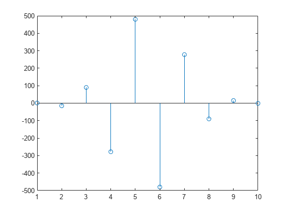
 1   -10    35   -52    35   -10     1

R = 1×10 single row vector

 1   -15    90  -278   480  -480   278   -90    15    -1

stem(R); % Plot the result

Figure contains an axes object. The axes object contains an object of type stem.

A Program That Works for Either Single or Double Precision

Now let's look at a function to compute enough terms in the Fibonacci sequence so the ratio is less than the correct machine epsilon (eps) for datatype single or double.

% How many terms needed to get single precision results? fibodemo('single')

% How many terms needed to get double precision results? fibodemo('double')

% Now let's look at the working code. type fibodemo

function nterms = fibodemo(dtype) %FIBODEMO Used by SINGLEMATH demo. % Calculate number of terms in Fibonacci sequence.

fcurrent = ones(dtype); fnext = fcurrent; goldenMean = (ones(dtype)+sqrt(5))/2; tol = eps(goldenMean); nterms = 2; while abs(fnext/fcurrent - goldenMean) >= tol nterms = nterms + 1; temp = fnext; fnext = fnext + fcurrent; fcurrent = temp; end

Notice that we initialize several of our variables, fcurrent, fnext, and goldenMean, with values that are dependent on the input datatype, and the tolerance tol depends on that type as well. Single precision requires that we calculate fewer terms than the equivalent double precision calculation.