Case study: Chirped-pulse ytterbium-doped fiber amplifier system (original) (raw)

Key questions:

• What pulse energies are feasible with a core-pumped Yb-doped fiber amplifier, and what are the crucial limitations?
• How strong can nonlinear phase shifts in the active fibers be until they prevent effective pulse compression?
• What kinds of trade-offs do we encounter in the design of chirped-pulse fiber amplifier systems?

Definition of Task

Figure 1: Evolution of the temporal pulse shape in a chirped-pulse amplifier.

As fiber-based ultrafast amplifiers are typically limited by nonlinear optical effects, one requires the principle of chirped-pulse amplification (CPA) to reach reasonably high pulse energies. Still, nonlinear effects are usually limiting the performance: due to the small effective mode area and long length of an active fiber (compared to that of a laser crystal), they become significant even for moderate peak powers. Designing such an amplifier system and exploring the limitations and involved trade-offs is not a trivial task, but you can a lot on those things in this article.

We consider unchirped Gaussian input pulses with 100 fs duration at 1040 nm. We will stretch these to a duration of 100 ps, exploring different options to do that. (Stronger stretching is possible, but becomes increasingly difficult.) The amplification should be done in a core-pumped Yb-doped large mode area fiber with 1000 μm2 mode area (which is a large but not extreme value). We will investigate how strong nonlinear phase shifts we can tolerate to still achieve effective pulse compression. Also, the required input pulse energy will need to be considered.

For the modeling, we use the software RP Fiber Power, which offers a Power Form titled “Fiber amplifier for ultrashort pulses”. We can just fill in all the parameters, including those for configuring some diagrams.

Representation of the Input Pulse

A Gaussian input pulse could normally be numerically represented with a rather short time trace, containing e.g. 28 = 256 complex amplitudes. However, for subsequent dispersive stretching to 100 ps, we need a long time trace with a width around 400 ps. In order to still have sufficient temporal resolution, we then need to have 214 or 215 amplitudes. This leads to a substantially increased computational load. Still, this is feasible with an ordinary PC, particularly when efficient software is used. Typically, one simulation run takes a couple of seconds.

Estimating the Possible Output Pulse Energy

The stretched pulse has a much reduced peak power, but that will grow again during amplification. Substantial nonlinear effects will take place if the output pulse energy reaches a peak power of the order of 50 kW, assuming a total fiber length of at most a few meters, a large mode area (an order of magnitude more than for a standard single-mode fiber) and considering that the highest peak power is reached only near the output end. (For such parameters, we expect a couple of radians of nonlinear phase shift.) That peak power of 50 kW combined with a stretched pulse duration of 100 ps results in an output pulse energy of 5 μJ. If we would go significantly beyond that, we must expect detrimental nonlinear effects.

We should also consider gain saturation. Significant gain saturation is good in the sense that we extract a substantial part of the energy which is initially stored in the amplifier. However, we should not overdo it. So we should calculate the saturation energy of the fiber: {E_{\rm sat}} = \frac{h\nu }{\sigma _{\rm em} + \sigma _{\rm abs}} A_{\rm eff}$$

Due to the large mode area, this is relatively large; for 1040 nm, we calculate 281 μJ. With our targeted output pulse energy being well below that, we can expect a moderate amount of gain saturation. This already tells us that we will be able to extract a significant but still relatively small part of the stored energy with one pulse since nonlinearities and not gain saturation will set the limit for the pulse energy.

Required Input Pulse Energy

If the gain of an amplifier becomes too high, we have high power losses due to amplified spontaneous emission (ASE). For a fiber amplifier, having a gain bandwidth of tens of nanometers, that becomes a problem when the gain reaches the order of 40 dB.

For a large mode area fiber, we actually like to work with less than that. One would then rather use two amplifier stages: a low-power preamplifier with e.g. 30 dB and a power amplifier with large mode area for another 10 dB.

With 40 dB overall gain, we then require an input pulse energy of 5 nJ. For a passively mode-locked solid-state bulk laser, this is feasible; with a typical pulse repetition rate of 100 MHz, it implies 100 MHz · 5 nJ = 500 mW average output power. However, for a mode-locked fiber laser it is already pretty high, although not impossible. It is just not easy to design such a fiber laser. Furthermore, a simple method of dispersive pulse stretching in a long fiber won't work at that high peak power level, as we will see.

In this situation, we see basically two different technical routes:

• We can use a mode locked laser with 5 nJ or even 50 nJ pulse energy (a bulk laser then being the simplest solution) in combination with a pulse stretcher which can handle that peak power — for example, a chirped volume Bragg grating.
• Alternatively, we can start with a much lower pulse energy of e.g. 0.1 nJ, stretch the pulses simply with a long passive fiber, and construct a fiber amplifier with rather high gain. For limiting ASE, spectral filtering between the stages is not a very effective solution, since the pulses are rather broadband. Also, polarization filtering could only contribute 3 dB attenuation. The only really effective way is to use a fast optical switch between the stages, which opens only for a short time when the input pulse enters the system.

Before deciding for an option, we consider the details of pulse stretching:

Dispersive Pulse Stretching

The theoretically simplest kind of dispersive stretching is with second-order dispersion only. We quickly find that we need to enter a GDD of 3.6 ps2 = 3'600'000 fs2 for stretching the pulses from 100 fs to a duration (FWHM) of 100 ps. We will see what options we have to realize that in practice.

Pulse Stretching in a Fiber

We can try to which extent the pulse stretching would be feasible with a sufficiently long passive single-mode fiber. For this, we use the Power Form “Passive fiber for ultrashort pulses”. We define a germanosilicate fiber with a core diameter of 8 μm and a numerical aperture of 0.093. With these parameters, it is in the single-mode regime (V-number = 2.26). The calculated group velocity dispersion is 20'677 fs2/m at 1040 nm. So the required 3'600'000 fs2 are provided by a few hundred meters of fiber, which is feasible (and also does not involve excessive propagation losses).

However, we should consider not only higher-order dispersion, but also the effect of the Kerr nonlinearity of the fiber. Therefore, we now numerically simulate the pulse propagation in that fiber, first for a low input pulse energy of 0.1 nJ. We find that the required pulse duration of 100 ps is reached after 120 m of that fiber — somewhat less than one would naively expect, since the Kerr nonlinearity provides additional spectral broadening: the spectral width increases moderately from 15.9 nm to 23.3 nm. That should not cause trouble for subsequent pulse compression; we can simulate that, e.g. simply using a constant GDD, where we reach 218 fs, or with dispersion up to third order, resulting in a compressed pulse duration of 82.7 fs. This is even less than the input pulse duration. The temporal and spectral pulse shapes are very smooth, i.e., without any wiggles as occur with dominant self-phase modulation:

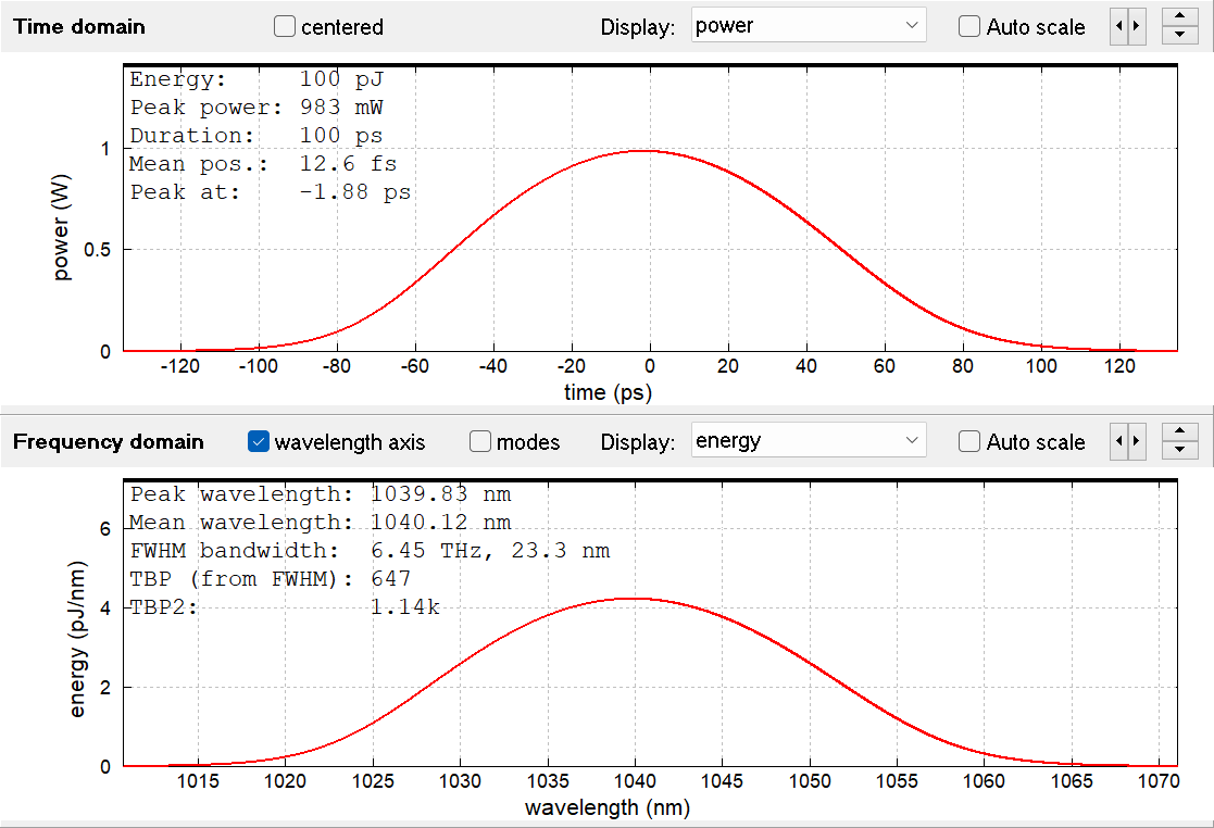
Figure 2: 0.1-nJ pulse after dispersive stretching in 120 m of fiber.

For a higher input pulse energy of 1 nJ, the initial peak power is 9.4 kW, making the nonlinear effect accordingly stronger. The pulse already broadens to 1.7 ps after 1 m, or 18.8 ps after 10 m. The desired duration of 100 ps is achieved after 52.5 m. The compressed pulse is at 163 fs with second-order dispersion only, or 40.7 fs with dispersion up to third order. Apparently, third-order dispersion gets more important for higher pulse energies. The spectral width expanded to 53.4 nm, but still with a very smooth spectral shape:

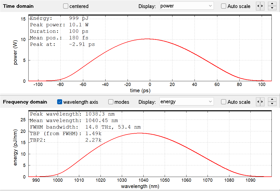
Figure 3: 1-nJ pulse after dispersive stretching in 52.5 m of fiber.

With 3-nJ pulses, it still works, giving us 100-ps pulses after 32 m:

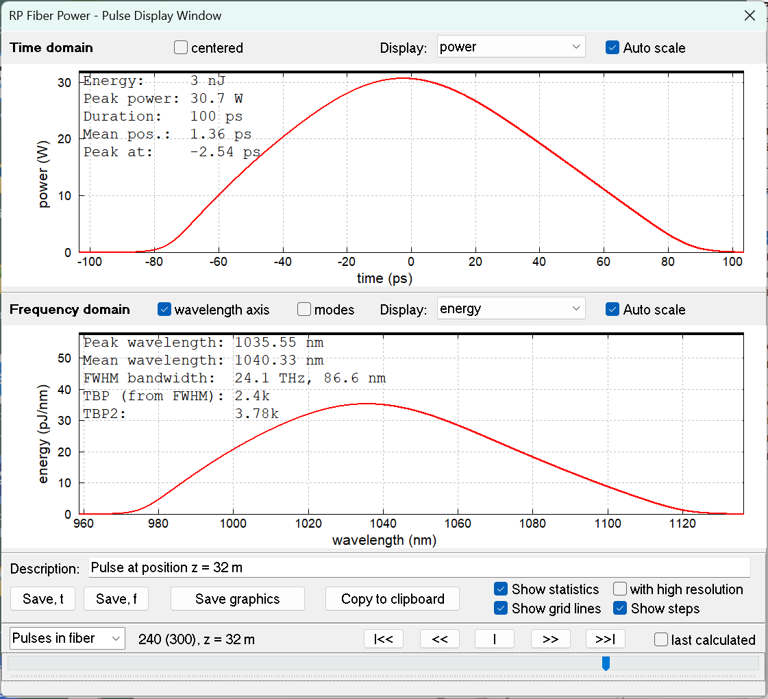
Figure 4: 3-nJ pulse after dispersive stretching in 32 m of fiber.

However, the spectrum now becomes really broad, going far beyond the region with good gain from ytterbium. Although we could directly compress these pulses to 29.5 fs, we would lose a lot of the bandwidth during amplification. It is hard to determine a safe limit without more detailed simulations of various cases (although including the amplifier and the compressor), but so far it seems that we should limit ourselves to the order of 1 nJ input energy if we want to use a passive fiber as pulse stretcher.

We could save any simulated pulse after the stretcher fiber to a file; from that, we could later load the pulse again as the input pulse for the amplifier simulation.

Pulse Stretching with a Chirped Volume Bragg Grating

An alternative method of pulse stretching with much weaker nonlinear effects (easily working for microjoule pulses) is based on a chirped volume Bragg grating. The basic idea is relatively simple: the Bragg wavelength of such a grating varies smoothly, so that different parts of the spectrum are reflected at different locations and thus experience different group delays. Well, this simple picture is really over-simplified, as the article on chirped mirrors explains, where we have essentially the same issues, just in a quite different parameter regime. But we can use this picture for a very rough estimate:

• Within 1 ns, light travels over roughly 20 cm in an optical glass with refractive index 1.5.
• For a time delay difference of 100 ps, we thus need a grating length of at least 1 cm. (Note the double pass.)
• Actually, we need time delays going somewhat beyond 100 ps, as we have smooth spectral distributions. A length of the order of 2 to 3 cm should be suitable.

It just requires rather high precision of fabrication to make such gratings; otherwise, one would easily get a more complicated frequency dependence of the group delay, implying strong higher-order dispersion which could spoil the pulses. For stronger stretching, that would become accordingly more challenging.

Pulse Stretching with a Pair of Diffraction Gratings

A classical method is based on a pair of diffraction gratings:

• The first grating disperses the optical frequency components to different angles (directions).
• After the second grating, the frequency components all travel in the same direction, but laterally displaced.
• When the light is reflected back, finally all frequency components travel together again, but have experienced different phase shifts and group delays.

That way, one can generate a large amount of anomalous dispersion — or normal dispersion, if one uses two lenses between the gratings in addition. Nonlinear effects are certainly negligible in our parameter regime.

In any case, such grating pulse stretchers also cause some amount of higher-order dispersion — dependent on the detailed configuration (including the number of lines per millimeter, the distance between gratings, and the incidence angles), so that there is some scope for optimization.

The Amplifier Design

Having explored the options for pulse stretching, we now decide on the overall amplifier architecture. In this case study, we want to focus on the issues related to the active fiber. Therefore, we now simply assume that we could somehow stretch the pulses by application of second-order dispersion only, and without causing additional nonlinear effects. We then get some nonlinear phase changes as well as gain narrowing in the amplifier fiber and can check how far the amplified pulses can still be compressed. Further, we assume that we can start with a relatively large input pulse energy of 50 nJ (after stretching to 100 ps duration), so that 20 dB gain — easily achievable with a single amplifier stage — are sufficient for getting to the 5-μJ regime, where we anticipate that nonlinear effects will start to become substantial.

Using a Single-mode Amplifier Fiber

In the simulation model, we set the parameters for a generic Yb-doped fiber with the large effective mode area of 1000 μm2. (Alternatively, we could use a parameter set of some commercially available fiber.) We assume a Yb doping density of 1025 m−3, leading to efficient pump absorption within a few meters of fiber (also depending on the degree of Yb excitation).

For simplicity, we further assume that the fiber is initially in the pumped state, i.e., that it is pumped over a sufficiently long time to reach the steady state before the input pulse comes. (We could later investigate repetitive operation for a given pulse repetition rate, but the specific aspects of that are not at the core of our interest here.)

We then quickly find that by pumping 2 m of that fiber with 2 W (in backward direction) at 940 nm, we would get to 5.1 μJ output pulse energy. Note that 2 W pump power injected into a single-mode fiber is pretty high, although not completely unrealistic. It would be substantially easier to get high pump powers into a double-clad fiber, but there we have less pump absorption, thus require a substantially longer fiber length, which in turn increases the nonlinear phase shifts. So for now we stick to the single-mode fiber approach and investigate the obtained pulses in the time and wavelength domain:

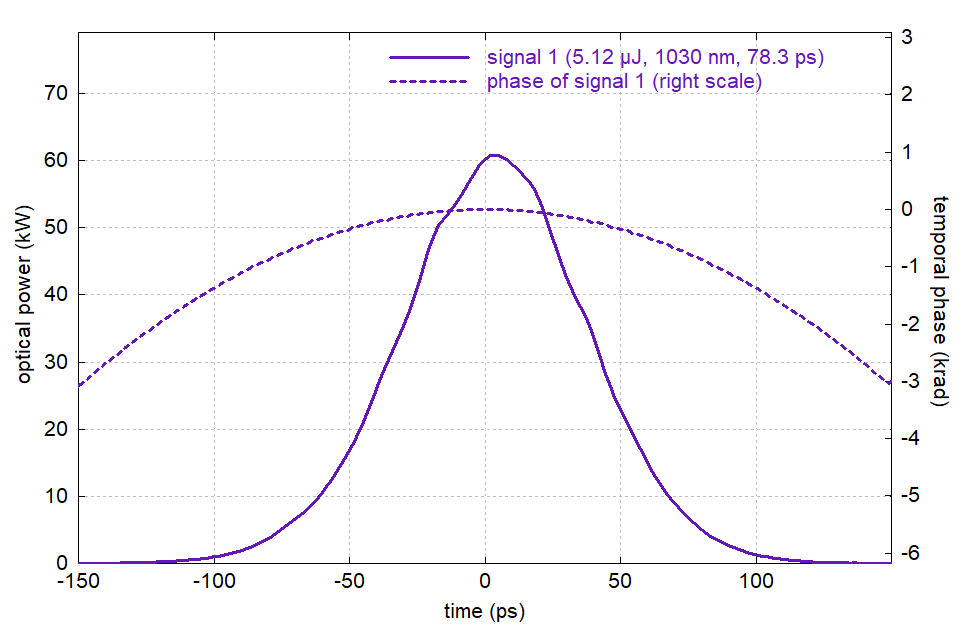
Figure 5: Amplified pulse in the time domain.

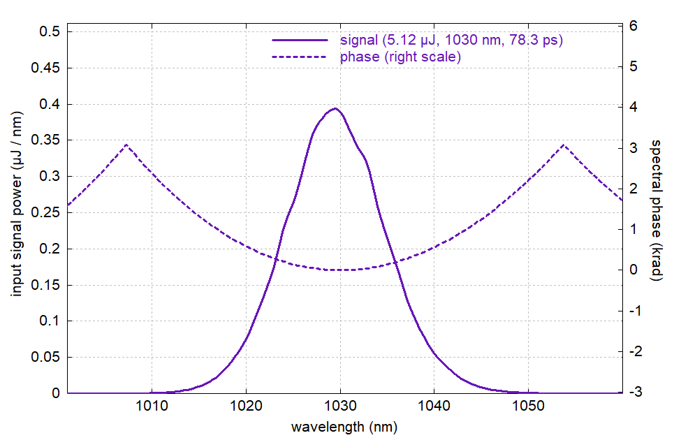
Figure 6: Amplified pulse in the wavelength domain. (The strong deviation from a parabolic phase profile in the extreme wings is a numerical artifact, which could be avoided with increased spectral resolution but is not relevant for our case.)

The pulse duration became significantly reduced from 100 ps to 78.3 ps. This is because for the chirped pulse, the temporal wings correspond to the spectral wings, which get less gain due to the limited gain bandwidth. (The trailing wing also gets somewhat less gain due to gain saturation.) Note also that the spectral peak moved from 1040 nm to 1030 nm, where the gain is highest. (That would be different for a double-clad fiber, which is typically operated at lower Yb excitation levels and thus has its gain maximum at longer wavelengths.) The output peak power is at 60.8 kW, which causes significant though not excessive nonlinear phase changes near the output end of the amplifier fiber. Note that we cannot see those in the diagram since the large spectral phase values (order of a kiloradian) are still dominated by the pulse stretching.

We then try temporal compression with numerically optimized dispersion of second and third order:

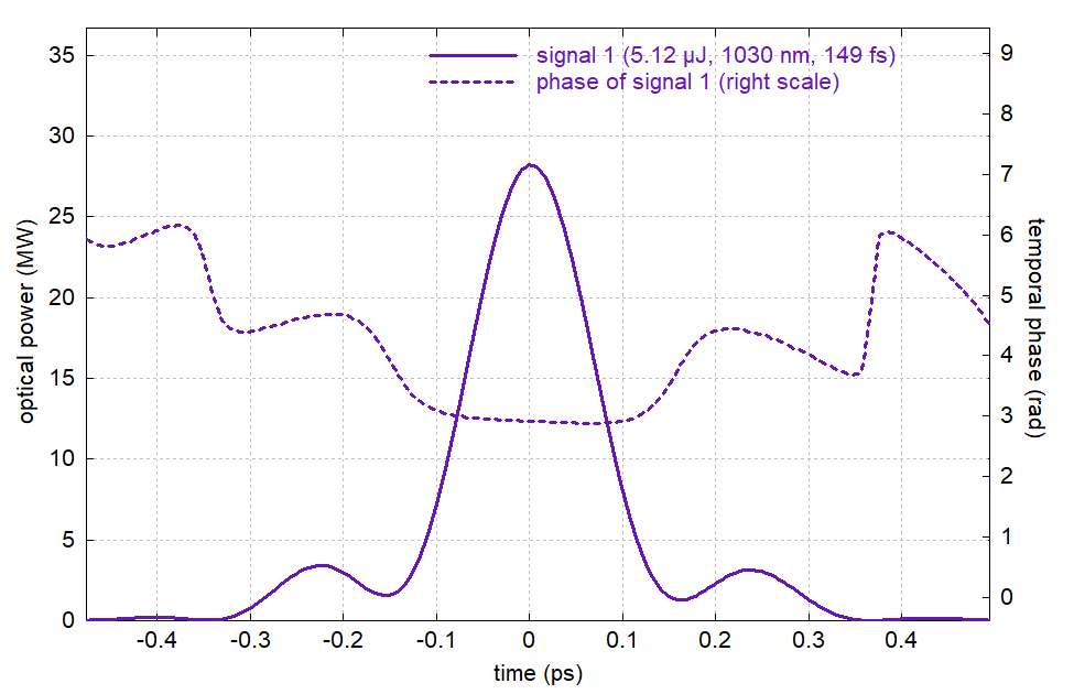
Figure 7: The compressed pulse (for dispersion up to third order) in the time domain.

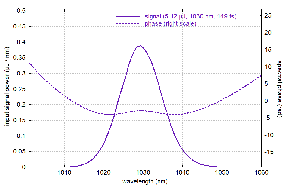
Figure 8: The compressed pulse in the wavelength domain.

The compressed pulse duration of 149 fs — 49% longer than the initial pulse duration — is limited by two issues:

• Spectral narrowing (gain narrowing) in the amplifier has reduced the FWHM bandwidth to 12.3 nm.
• The quality of compression (which we recognize from the spectral phase) is not perfect. Obviously, the nonlinear phase shifts in the amplifier has some negative side effects on the compression. (If one turns that off in the simulation, the compression yields 119-fs pulses.)

We can get substantially better by optimizing the compressor dispersion up to fourth order (which is of course technically more difficult in practice):

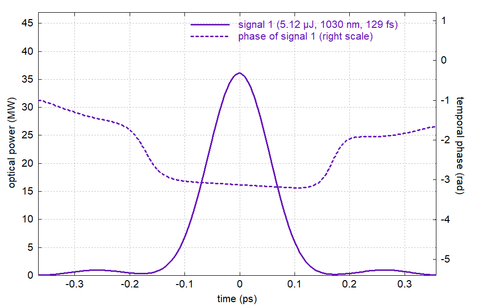
Figure 9: The compressed pulse (for dispersion up to fourth order) in the time domain.

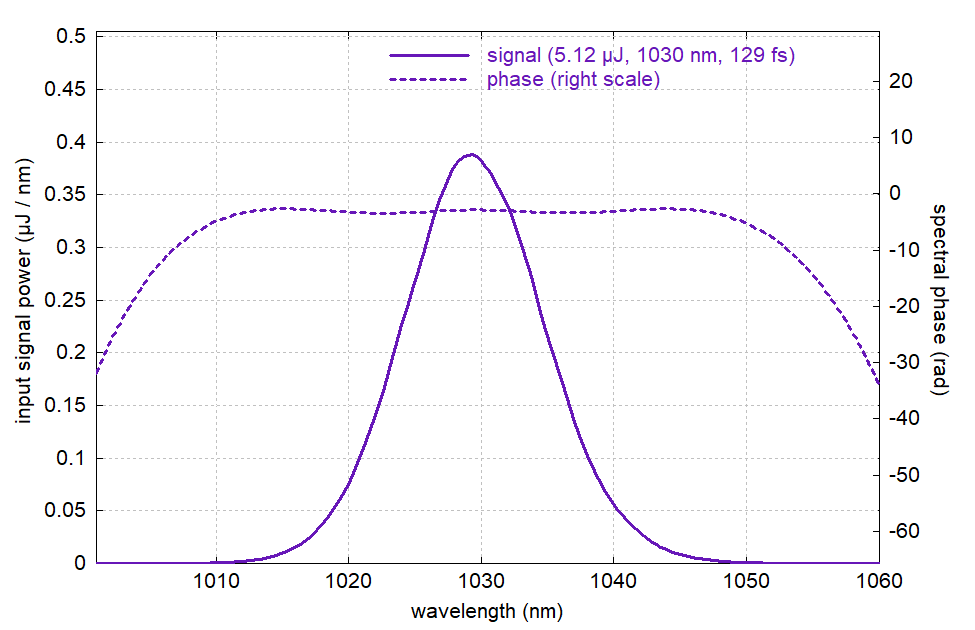
Figure 10: The compressed pulse in the wavelength domain.

The compressed pulse duration is reduced to 129 fs, but this is still worse than without the nonlinear effect in the amplifier, and also that does not take into account the side peaks of the pulse, which may be detrimental for an application.

So these results confirm the initial expectation that the nonlinear phase shifts caused in the amplifier fiber should really not exceed a few radians. This may be surprising, given that the applied dispersive phase shifts amount to a few thousand radians, but note that while the pulse stretcher applies a parabolic spectral phase shift, that shape is substantially different for the nonlinear phase shifts.

Before we go further, we quickly check whether stimulated Raman scattering could also have an influence. That has previously been ignored in the simulation, but can simply turn it on. However, the results are quite precisely the same with that effect; we do not have sufficiently strong nonlinear phase shifts to make Raman scattering relevant.

Using a Double-clad Fiber

Next, we can try how it works out with a double-clad fiber. So we now assume a pump cladding with 125 μm diameter, increase the fiber length to 10 m and the pump power to 3.3 W. (For such a large pump cladding, applying even much more pump power would be easy, using some fiber-coupled diode bar.) One may be surprised that with increasing the fiber length by far less than the ratio of pump cladding to core area, we still get reasonably efficient pump absorption — this is because we now have less pump saturation, associated with a lower fractional Yb excitation density. However, the nonlinear effects are still too strong for that fiber length: although we can well amplify the pulses to around 5 μJ and more, compression gets difficult:

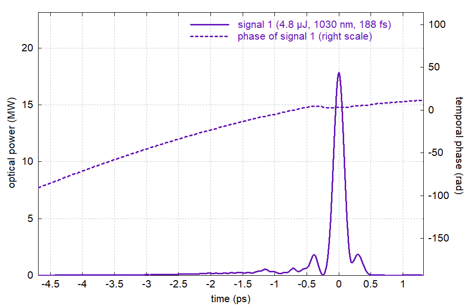
Figure 11: Compressed pulse from 10 m long double-clad fiber.

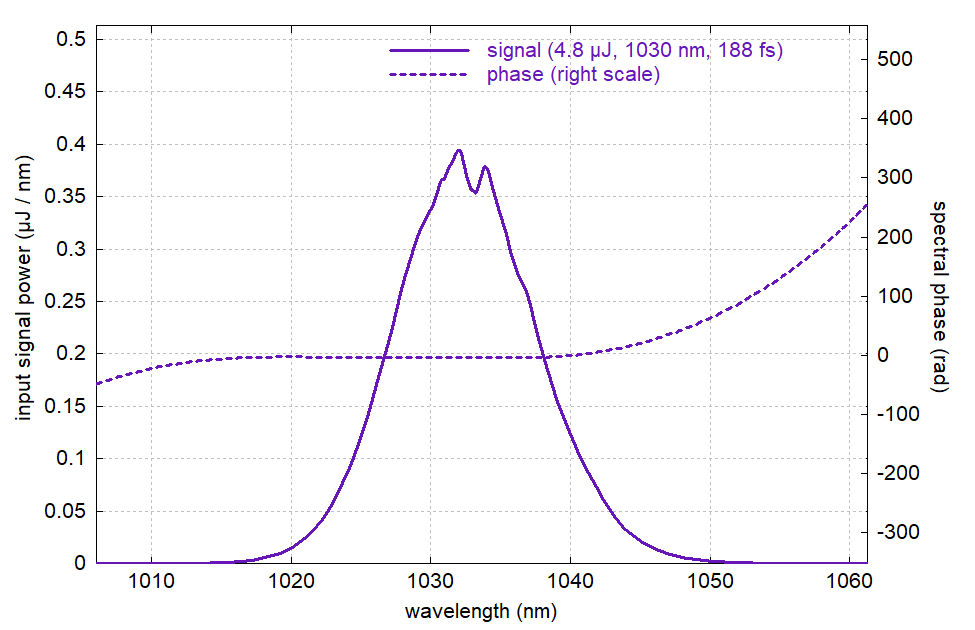
Figure 12: Spectrum of compressed pulse from 10 m long double-clad fiber.

Note that the software did not fail to apply sufficient third-order dispersion, as the remaining spectral phase may seem to suggest. Indeed, the spectral phase got reasonably flat throughout much of the spectrum, but then deviates substantially in the wings, particularly the one on the long wavelength side. It only gets better if we optimize dispersion up to the 6th order:

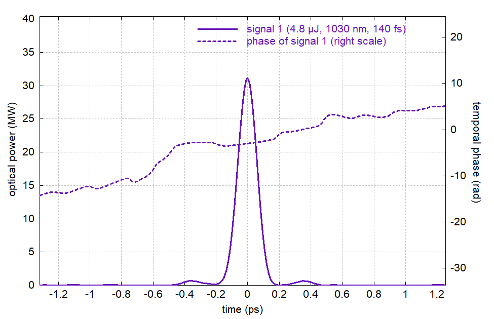
Figure 13: Compressed pulse from 10 m long double-clad fiber.

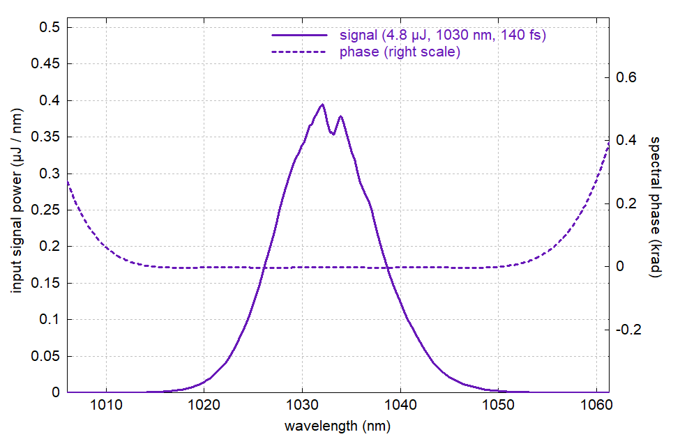
Figure 14: Spectrum of compressed pulse from 10 m long double-clad fiber.

That is possible in principle, but really not so easy to realize in practice.

Another option is to use a much shorter fiber (e.g. 2 m length), accepting that pump absorption will be quite incomplete, and inefficiently using substantially more pump input power. Simulations show that with 10.5 W pump power we now get 5.12 μJ out:

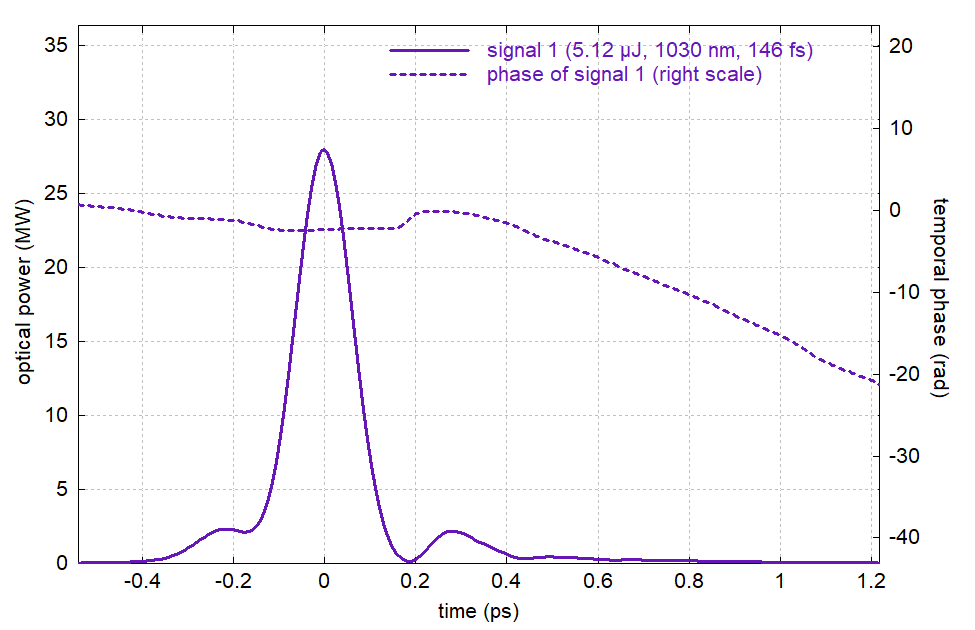
Figure 15: Compressed pulse from 2 m long double-clad fiber.

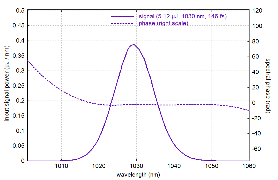
Figure 16: Spectrum of compressed pulse from 2 m long double-clad fiber.

For compression, we only used dispersion up to third order. Compared to the previous case with 10 m length, the compression works significantly better. So we can to some extent trade the complexity of pulse compression against the required pump power.

Additional Details

Various additional details, going beyond the scope of this case study, may be interesting in practical cases. Some examples:

• One may employ a flexible kind of pulse stretcher based on diffraction gratings and a spatial light modulator. It would then be interesting to test whether we can tolerate substantially larger nonlinear phase changes by properly pre-destorting the input pulses.
• In a case where we want to start with a relatively low pulse energy and need accordingly more gain, one would need to investigate how to sufficiently suppress ASE in the amplifier system. For example, how fast would an optical switch between the amplifier stages need to be, and how much would the output pulses be accompanied by an ASE background.
• One could check with what precision the pump power needs to be kept constant to achieve effective pulse compression, and what effects fluctuations in the input pulse energy would have.

Many additional details like those could also be well addressed with numerical simulations.

Conclusions

We can extract a number of conclusions from this investigation:

• There are different methods of pulse stretching, which have specific advantages and limitations. Using a long passive fiber, for example, is a simple option but works well only for quite low pulse energies.
• Such issues are related to how much input pulse energy we can use, and how much gain the amplifier then needs to have. Some trade-offs results from that. We may, for example, either decide for a simple pulse source and stretching technique but use a more complicated two-stage fiber amplifier. Alternatively, we may combine a higher-energy seed laser with a different technique for pulse stretching and a simple single-stage amplifier.
• Even when using an active fiber with substantial mode area and reasonable long stretched pulses, nonlinear effects are quite limiting for the performance — even more so if a double-clad fiber is to be used, which has to be longer (or will not efficiently absorb the applied pump power). The nonlinear phase shifts should be limited to a few radians, even if the phase changes associated with pulse stretching are far stronger than that.
• With refined pulse compression techniques, also addressing higher orders of dispersion, we can accept somewhat stronger nonlinear phase shifts, but this is more difficult to realize in practice.
• Developing such an amplifier system without numerical simulations — simply with trial & error — would be highly inefficient, since a number of important questions could not be clarified before ordering the components, and also not easily answered based on experimental results. With suitable simulation software, being sufficiently flexible and easy to handle, a reasonable amplifier design and its limitations are found far more quickly and with lower cost. Working with that also leads to a far deeper understanding and possibly more creative technical solutions.

Video

Here, you can see how the simulations for this case study were done with our software RP Fiber Power:

Your browser does not support the video tag. However, you can download the video file.