Covariance Structure (original) (raw)
This vignette details the different covariance structures available in clustTMB.
Random Effect Covariance Matrices
| Covariance | Notation | No..of.Parameters | Data.requirements |
|---|---|---|---|
| Spatial GMRF | gmrf | 2 | spatial coordinates |
| AR(1) | ar1 | 2 | unit spaced levels |
| Rank Reduction | rr(random = H) | JH - (H(H-1))/2 | |
| Spatial Rank Reduction | rr(spatial = H) | 1 + JH - (H(H-1))/2 | spatial coordinates |
Spatial GMRF
clustTMB fits spatial random effects using a Gaussian Markov Random Field (GMRF). The precision matrix,QQ, of the GMRF is the inverse of a Matern covariance function and takes two parameters: 1)κ\kappa, which is the spatial decay parameter and a scaled function of the spatial range,ϕ=8/κ\phi = \sqrt{8}/\kappa, the distance at which two locations are considered independent; and 2)τ\tau, which is a function ofκ\kappaand the marginal spatial varianceσ2\sigma^{2}:
τ=12πκσ.\tau = \frac{1}{2\sqrt{\pi}\kappa\sigma}.The precision matrix is approximated following the SPDE-FEM approach[@Lindgren2011], where a constrained Delaunay triangulation network is used to discretize the spatial extent in order to determine a GMRF for a set of irregularly spaced locations, i$.
ωi∼GMRF(Q[κ,τ])\omega_{i} \sim GMRF(Q[\kappa, \tau])
Spatial Example
Prior to fitting a spatial cluster model with clustTMB, users need to set up the constrained Delaunay Triangulation network using the R package, fmesher. This package provides a CRAN distributed collection of mesh functions developed for the package, R-INLA. For guidance on setting up an appropriate mesh, see Triangulation details and examples and Tools for mesh assessment from
In this example, the following mesh specifications were used:
## Loading required namespace: INLA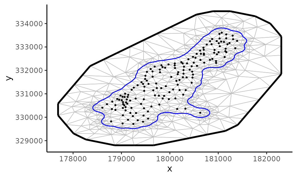
Coordinates are converted to a spatial point dataframe and read into the clustTMB model, along with the mesh, using the spatial.list argument. The gating formula is specified using the gmrf() command:
Loc <- sf::st_as_sf(loc, coords = c("x", "y"))
mod <- clustTMB(
  response = meuse[, 3:6],
  family = lognormal(link = "identity"),
  gatingformula = ~ gmrf(0 + 1 | loc),
  G = 4, covariance.structure = "VVV",
  spatial.list = list(loc = Loc, mesh = meuse.mesh)
)
## intercept removed from gatingformula
## when random effects specified## spatial projection is turned off. Need to provide locations in projection.list$grid.df for spatial predictionsModels are optimized with nlminb(), model results can be viewed with nlminb commands:
# Estimated fixed parameters
mod$opt$par
## betag betag betag betad betad betad betad
## 0.1778785 0.5710390 0.1653808 2.0157770 4.3160891 5.4259812 6.7095828
## betad betad betad betad betad betad betad
## 1.0064910 3.6030481 5.2113125 6.2155339 0.1259838 3.1475098 4.2016963
## betad betad betad betad betad theta theta
## 5.2523458 -1.4361518 3.1132965 4.2118628 5.1996580 -1.2100719 -2.9055373
## theta theta theta theta theta theta theta
## -1.2794893 -1.2502242 -2.5624052 -3.1154930 -2.2459437 -2.3607707 -1.8075154
## theta theta theta theta theta theta theta
## -4.0486948 -2.6845241 -3.0661981 -2.4648459 -3.3381189 -2.7804368 -2.6686023
## ln_kappag
## -5.9132622# Minimum negative log likelihood
mod$opt$objective## [1] 2318.892Gating Network Examples
When random effects,𝕦\mathbb{u}, are specified in the gating network, the probability of cluster membershipπi,g\pi_{i,g}for observationiiis fit using multinomial regression:
η,g=Xβ,g+𝕦,gℼ,g=exp(η,g)∑g=1Gexp(η,g)\begin{align} \mathbb{\eta}_{,g} &= X\mathbb{\beta}_{,g} + \mathbb{u}_{,g} \\ \mathbb{\pi}_{,g} &= \frac{ exp(\mathbb{\eta}_{,g})}{\sum^{G}_{g=1}exp(\mathbb{\eta}_{,g})} \end{align}