The iraceplot package: User Guide (original) (raw)
In the following, we provide an example how the functions implemented in this package can be used to visualize the information generated by irace.
Configurations
Once irace is executed, the first thing you might want to do is to visualize how the best configurations look like. You can do this with the parallel_coord method:
The plot shows by default the final elite configurations (last iteration), each line in the plot represents one configuration. The plot produced by parallel_coord can help you to both the distribution of the parameter values of a set of configurations and the common associations between these values. By default, the plot colors the lines using the number of instances evaluated by the configuration. You can use the color_by_instances argument to choose between coloring the lines by the number of instances executed or the last iteration the configurationwas executed on.
To visualize the configurations considered as elites in each iteration use the iterations option. You can select one or more iterations. For example, to select all iterations executed by irace:
parallel_coord(iraceResults, iterations=1:iraceResults$state$nbIterations,
               color_by_instances = FALSE)
You can also visualize all configurations sampled in one or more iterations disabling the only_elite option. For example, to visualize configurations sampled in iterations 1 to 9:
If you are looking for something more flexible and you would like to provide your own set of configurations, you can use the[plot_configurations()](../../reference/plot%5Fconfigurations.html) function. This function generates a parallel coordinates plot (similar to the ones generated by[parallel_coord()](../../reference/parallel%5Fcoord.html)) when provided with an arbitrary set of configurations and a parameter space object. The configurations must be provided in the format in which irace handles configurations: a dataframe with parameter in each column. For information about these formats, please chech the irace package user guide. As an example, this lines display all elite configurations:
all_elite <- iraceResults$allConfigurations[unlist(iraceResults$allElites),]
parameters <- iraceResults$scenario$parameters
plot_configurations(all_elite, parameters)
The parallel_cat function displays all configurations sampled in a set of iterations. The plot groups parameter values in intervals and thus, it can be useful to visualize more tendencies of association between parameters values. As in the previous functions you can use the iterations argument to select the iterations from which configurations should be selected. For example, to visualize configurations sampled on iterations 3, 4 and 5:
parallel_cat(irace_results = iraceResults, iterations = c(3,4,5) )## Warning in set(tabla, i = which(not_na), j = pname, value = bins): Coercing
## 'character' RHS to 'double' to match the type of column 5 named 'alpha'.## Warning in set(tabla, i = which(not_na), j = pname, value = bins): NAs
## introduced by coercion## Warning in set(tabla, i = which(is.na(tabla[[pname]])), j = pname, value =
## "NA"): Coercing 'character' RHS to 'double' to match the type of column 5 named
## 'alpha'.## Warning in set(tabla, i = which(is.na(tabla[[pname]])), j = pname, value =
## "NA"): NAs introduced by coercion## Warning in set(tabla, i = which(not_na), j = pname, value = bins): Coercing
## 'character' RHS to 'double' to match the type of column 6 named 'beta'.## Warning in set(tabla, i = which(not_na), j = pname, value = bins): NAs
## introduced by coercion## Warning in set(tabla, i = which(is.na(tabla[[pname]])), j = pname, value =
## "NA"): Coercing 'character' RHS to 'double' to match the type of column 6 named
## 'beta'.## Warning in set(tabla, i = which(is.na(tabla[[pname]])), j = pname, value =
## "NA"): NAs introduced by coercion## Warning in set(tabla, i = which(not_na), j = pname, value = bins): Coercing
## 'character' RHS to 'double' to match the type of column 7 named 'rho'.## Warning in set(tabla, i = which(not_na), j = pname, value = bins): NAs
## introduced by coercion## Warning in set(tabla, i = which(is.na(tabla[[pname]])), j = pname, value =
## "NA"): Coercing 'character' RHS to 'double' to match the type of column 7 named
## 'rho'.## Warning in set(tabla, i = which(is.na(tabla[[pname]])), j = pname, value =
## "NA"): NAs introduced by coercion## Warning in set(tabla, i = which(not_na), j = pname, value = bins): Coercing
## 'character' RHS to 'double' to match the type of column 8 named 'ants'.## Warning in set(tabla, i = which(not_na), j = pname, value = bins): NAs
## introduced by coercion## Warning in set(tabla, i = which(is.na(tabla[[pname]])), j = pname, value =
## "NA"): Coercing 'character' RHS to 'double' to match the type of column 8 named
## 'ants'.## Warning in set(tabla, i = which(is.na(tabla[[pname]])), j = pname, value =
## "NA"): NAs introduced by coercion## Warning in set(tabla, i = which(not_na), j = pname, value = bins): Coercing
## 'character' RHS to 'double' to match the type of column 9 named 'nnls'.## Warning in set(tabla, i = which(not_na), j = pname, value = bins): NAs
## introduced by coercion## Warning in set(tabla, i = which(is.na(tabla[[pname]])), j = pname, value =
## "NA"): Coercing 'character' RHS to 'double' to match the type of column 9 named
## 'nnls'.## Warning in set(tabla, i = which(is.na(tabla[[pname]])), j = pname, value =
## "NA"): NAs introduced by coercion## Warning in set(tabla, i = which(not_na), j = pname, value = bins): Coercing
## 'character' RHS to 'double' to match the type of column 10 named 'q0'.## Warning in set(tabla, i = which(not_na), j = pname, value = bins): NAs
## introduced by coercion## Warning in set(tabla, i = which(is.na(tabla[[pname]])), j = pname, value =
## "NA"): Coercing 'character' RHS to 'double' to match the type of column 10
## named 'q0'.## Warning in set(tabla, i = which(is.na(tabla[[pname]])), j = pname, value =
## "NA"): NAs introduced by coercion## Warning in set(tabla, i = which(not_na), j = pname, value = bins): Coercing
## 'character' RHS to 'double' to match the type of column 12 named 'rasrank'.## Warning in set(tabla, i = which(not_na), j = pname, value = bins): NAs
## introduced by coercion## Warning in set(tabla, i = which(is.na(tabla[[pname]])), j = pname, value =
## "NA"): Coercing 'character' RHS to 'double' to match the type of column 12
## named 'rasrank'.## Warning in set(tabla, i = which(is.na(tabla[[pname]])), j = pname, value =
## "NA"): NAs introduced by coercion## Warning in set(tabla, i = which(not_na), j = pname, value = bins): Coercing
## 'character' RHS to 'double' to match the type of column 13 named 'elitistants'.## Warning in set(tabla, i = which(not_na), j = pname, value = bins): NAs
## introduced by coercion## Warning in set(tabla, i = which(is.na(tabla[[pname]])), j = pname, value =
## "NA"): Coercing 'character' RHS to 'double' to match the type of column 13
## named 'elitistants'.## Warning in set(tabla, i = which(is.na(tabla[[pname]])), j = pname, value =
## "NA"): NAs introduced by coercion## Warning: Removed 408 rows containing non-finite outside the scale range
## (`stat_parallel_sets()`).## Warning: Removed 408 rows containing non-finite outside the scale range
## (`stat_parallel_sets_axes()`).
## Removed 408 rows containing non-finite outside the scale range
## (`stat_parallel_sets_axes()`).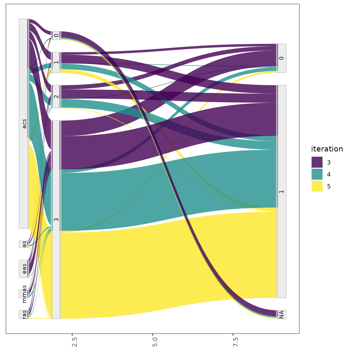
You can also adjust the number of value intervals that are displayed for each parameter using the n_bins parameter which by default is set to 3. Also, it is possible to select a subset of configurations using the id_configurations argument providing a vector a configuration ids.
Both in the parallel_coord and parallel_catfunctions parameters can be selected using the param_namesargument. For example to select parameters unparallel_cat:
parallel_cat(irace_results = iraceResults,
             param_names=c("algorithm", "localsearch", "dlb", "nnls"))
## Warning in set(tabla, i = which(not_na), j = pname, value = bins): Coercing
## 'character' RHS to 'double' to match the type of column 5 named 'alpha'.## Warning in set(tabla, i = which(not_na), j = pname, value = bins): NAs
## introduced by coercion## Warning in set(tabla, i = which(is.na(tabla[[pname]])), j = pname, value =
## "NA"): Coercing 'character' RHS to 'double' to match the type of column 5 named
## 'alpha'.## Warning in set(tabla, i = which(is.na(tabla[[pname]])), j = pname, value =
## "NA"): NAs introduced by coercion## Warning in set(tabla, i = which(not_na), j = pname, value = bins): Coercing
## 'character' RHS to 'double' to match the type of column 6 named 'beta'.## Warning in set(tabla, i = which(not_na), j = pname, value = bins): NAs
## introduced by coercion## Warning in set(tabla, i = which(is.na(tabla[[pname]])), j = pname, value =
## "NA"): Coercing 'character' RHS to 'double' to match the type of column 6 named
## 'beta'.## Warning in set(tabla, i = which(is.na(tabla[[pname]])), j = pname, value =
## "NA"): NAs introduced by coercion## Warning in set(tabla, i = which(not_na), j = pname, value = bins): Coercing
## 'character' RHS to 'double' to match the type of column 7 named 'rho'.## Warning in set(tabla, i = which(not_na), j = pname, value = bins): NAs
## introduced by coercion## Warning in set(tabla, i = which(is.na(tabla[[pname]])), j = pname, value =
## "NA"): Coercing 'character' RHS to 'double' to match the type of column 7 named
## 'rho'.## Warning in set(tabla, i = which(is.na(tabla[[pname]])), j = pname, value =
## "NA"): NAs introduced by coercion## Warning in set(tabla, i = which(not_na), j = pname, value = bins): Coercing
## 'character' RHS to 'double' to match the type of column 8 named 'ants'.## Warning in set(tabla, i = which(not_na), j = pname, value = bins): NAs
## introduced by coercion## Warning in set(tabla, i = which(is.na(tabla[[pname]])), j = pname, value =
## "NA"): Coercing 'character' RHS to 'double' to match the type of column 8 named
## 'ants'.## Warning in set(tabla, i = which(is.na(tabla[[pname]])), j = pname, value =
## "NA"): NAs introduced by coercion## Warning in set(tabla, i = which(not_na), j = pname, value = bins): Coercing
## 'character' RHS to 'double' to match the type of column 9 named 'nnls'.## Warning in set(tabla, i = which(not_na), j = pname, value = bins): NAs
## introduced by coercion## Warning in set(tabla, i = which(is.na(tabla[[pname]])), j = pname, value =
## "NA"): Coercing 'character' RHS to 'double' to match the type of column 9 named
## 'nnls'.## Warning in set(tabla, i = which(is.na(tabla[[pname]])), j = pname, value =
## "NA"): NAs introduced by coercion## Warning in set(tabla, i = which(not_na), j = pname, value = bins): Coercing
## 'character' RHS to 'double' to match the type of column 10 named 'q0'.## Warning in set(tabla, i = which(not_na), j = pname, value = bins): NAs
## introduced by coercion## Warning in set(tabla, i = which(is.na(tabla[[pname]])), j = pname, value =
## "NA"): Coercing 'character' RHS to 'double' to match the type of column 10
## named 'q0'.## Warning in set(tabla, i = which(is.na(tabla[[pname]])), j = pname, value =
## "NA"): NAs introduced by coercion## Warning in set(tabla, i = which(not_na), j = pname, value = bins): Coercing
## 'character' RHS to 'double' to match the type of column 12 named 'rasrank'.## Warning in set(tabla, i = which(not_na), j = pname, value = bins): NAs
## introduced by coercion## Warning in set(tabla, i = which(is.na(tabla[[pname]])), j = pname, value =
## "NA"): Coercing 'character' RHS to 'double' to match the type of column 12
## named 'rasrank'.## Warning in set(tabla, i = which(is.na(tabla[[pname]])), j = pname, value =
## "NA"): NAs introduced by coercion## Warning in set(tabla, i = which(not_na), j = pname, value = bins): Coercing
## 'character' RHS to 'double' to match the type of column 13 named 'elitistants'.## Warning in set(tabla, i = which(not_na), j = pname, value = bins): NAs
## introduced by coercion## Warning in set(tabla, i = which(is.na(tabla[[pname]])), j = pname, value =
## "NA"): Coercing 'character' RHS to 'double' to match the type of column 13
## named 'elitistants'.## Warning in set(tabla, i = which(is.na(tabla[[pname]])), j = pname, value =
## "NA"): NAs introduced by coercion## Warning: Removed 124 rows containing non-finite outside the scale range
## (`stat_parallel_sets()`).## Warning: Removed 124 rows containing non-finite outside the scale range
## (`stat_parallel_sets_axes()`).
## Removed 124 rows containing non-finite outside the scale range
## (`stat_parallel_sets_axes()`).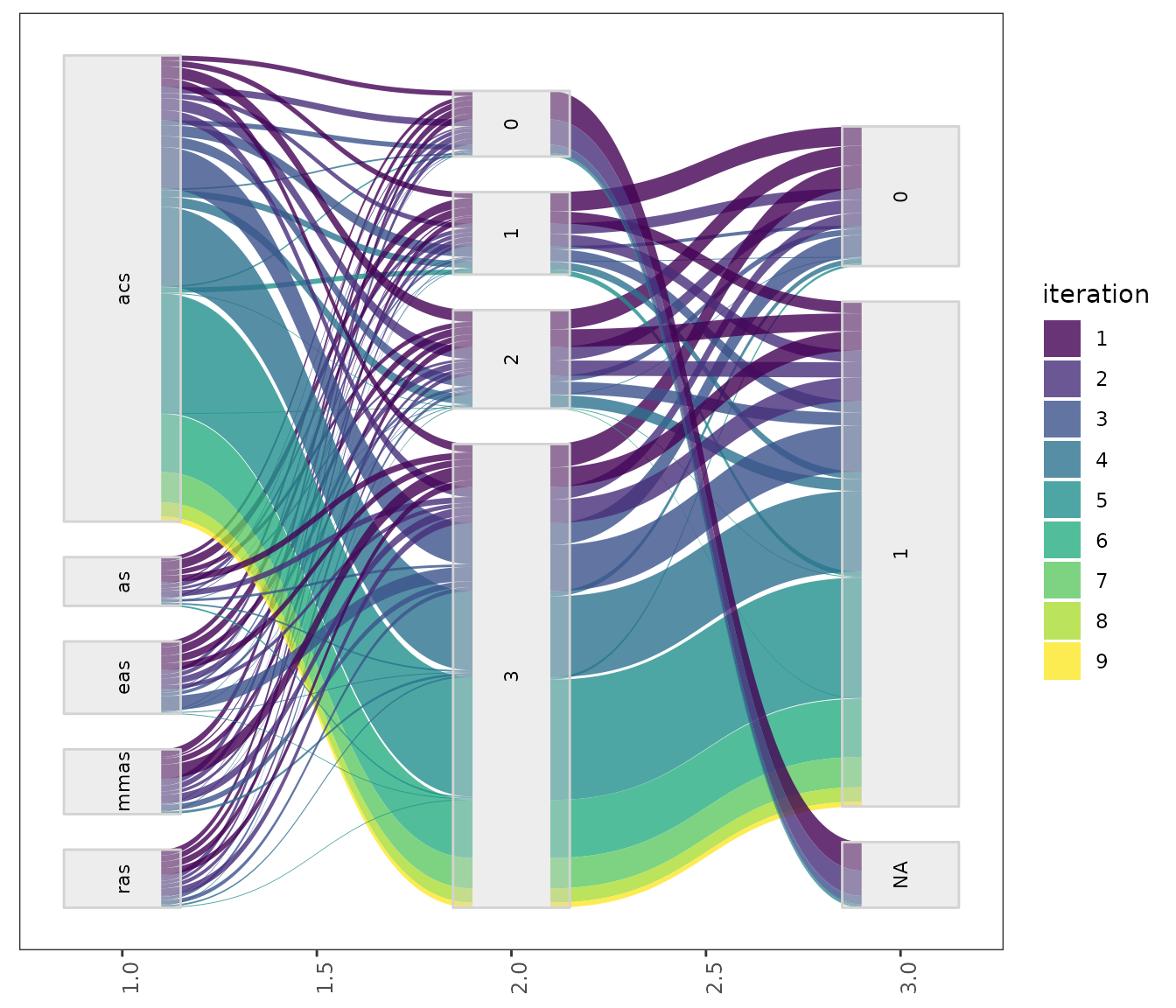
This setting is useful to visualize the association between parameters that, for example, seem to interact. For configuration scenarios that define a large number of parameters, it is impossible to visualize all parameters in one of these plots. If do not know which parameters to select, all parameters can be split in different plots using the by_n_param argument which specifies the maximum number of parameters to include in a plot. The functions will generate as many plots as needed to cover all parameters included.
Sampled values and frecuencies
The sampling_pie function creates a plot that displays the values of all configurations sampled during the configuration process. This plot can be useful to display the tendencies in the sampling in a simple format. As well as in thepreviousparallel_cat` plot, numerical parameters domains are discretized to be shown in the plot. The size of each parameter value in the plot is dependent of the number of configurations having that value in the configurations.
As in previous plots, you can select the parameters to display with the param_names argument and the number of intervals of each parameter with the n_bins argument. The generated plot is interactive, you can click in each parameter to display it independently.
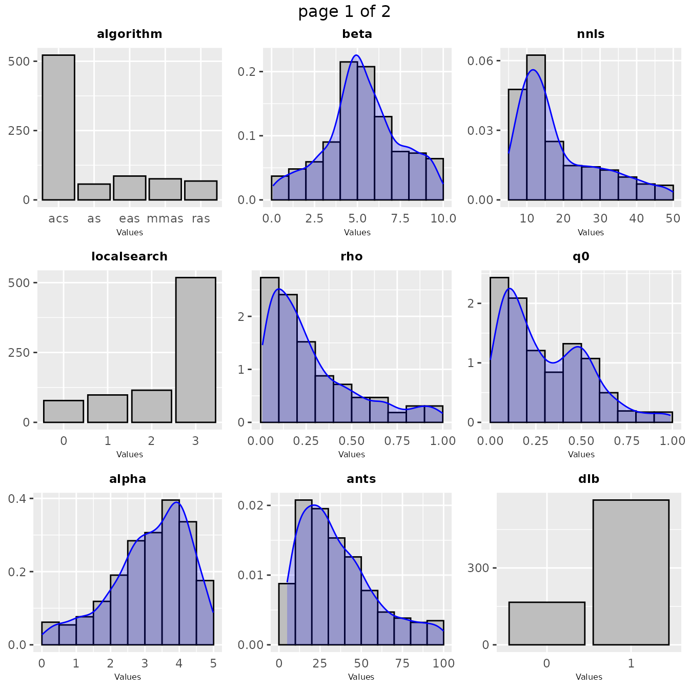
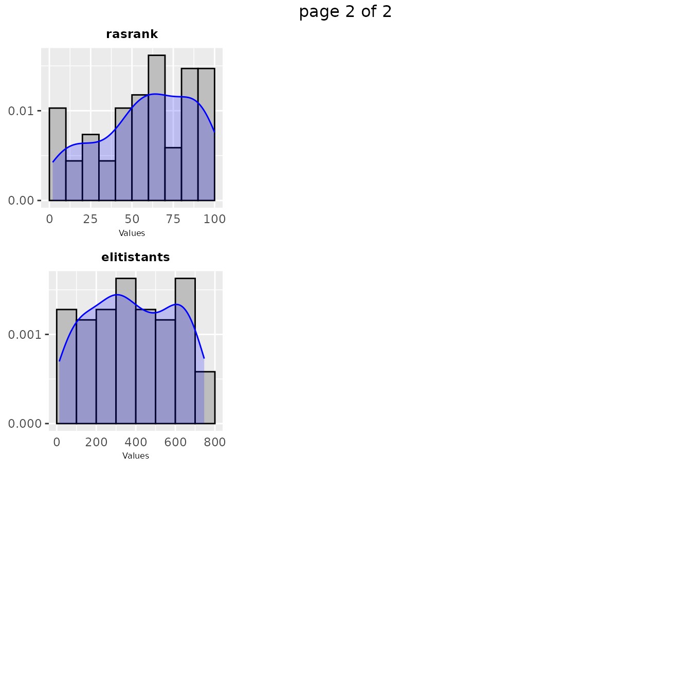
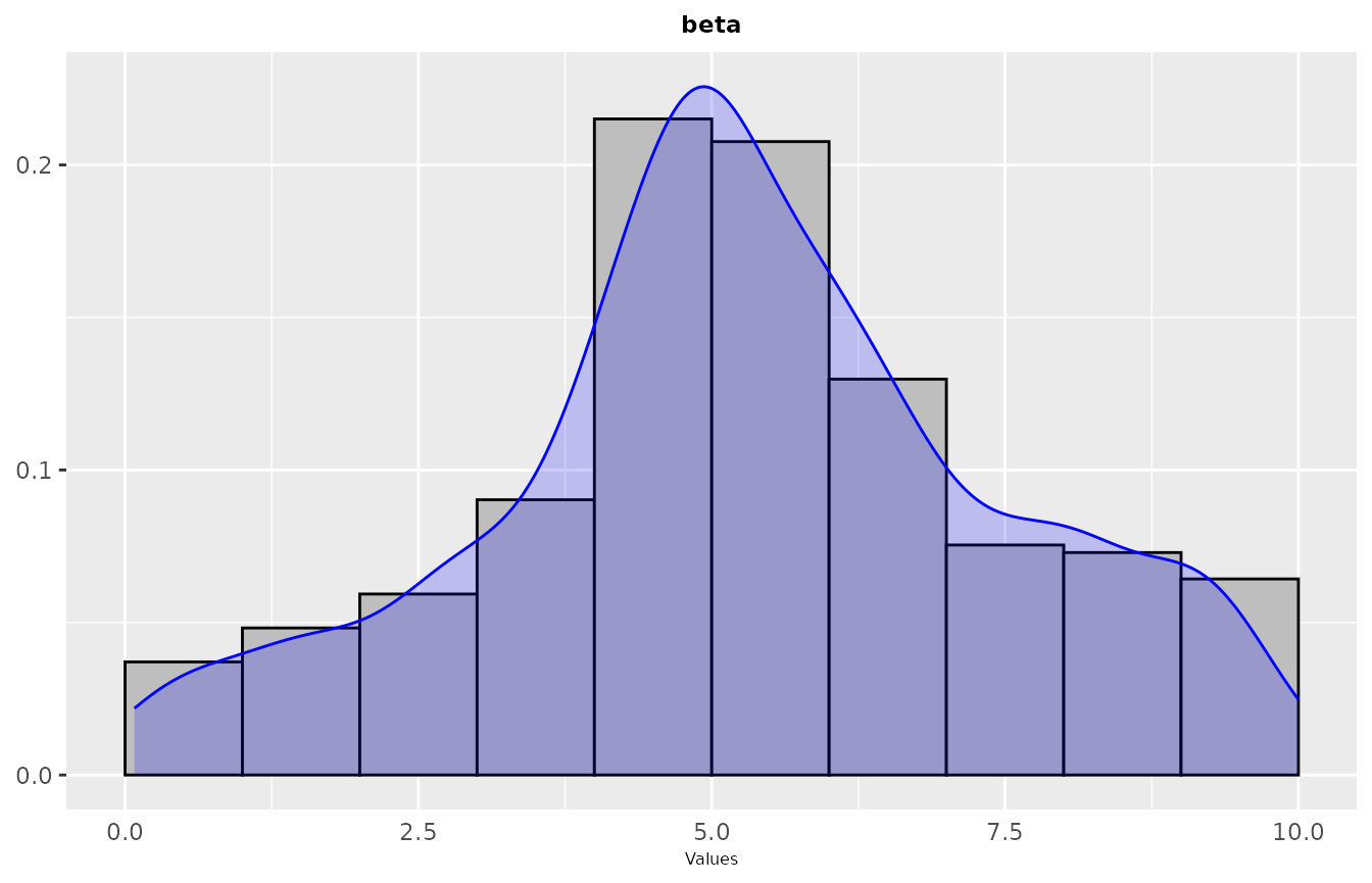
In some cases in might be interesting to have a look at the values sampled during the configuration procedure as a distribution. Such plot shows the areas in the parameter space where irace detected a high performance. A general overview of the distribution of sampled parameters values can be obtained with thesampling_frequencyfunction which generates frequency and density plots for the sampled values:
If you would like to visualize the distribution of a particular set of configurations, you can pass directly a set of configurations and a parameters object in the irace format to thesampling_frequency function:
The previous functions display the parameter frequency plots grouped by 9 plots, you can adjust this setting using the nargument. You can select the parameters to be displayed, with theparam_names argument. You can use these plots to ge a general idea of the area of the parameter space in which the sampling performed by irace was focused. For example:
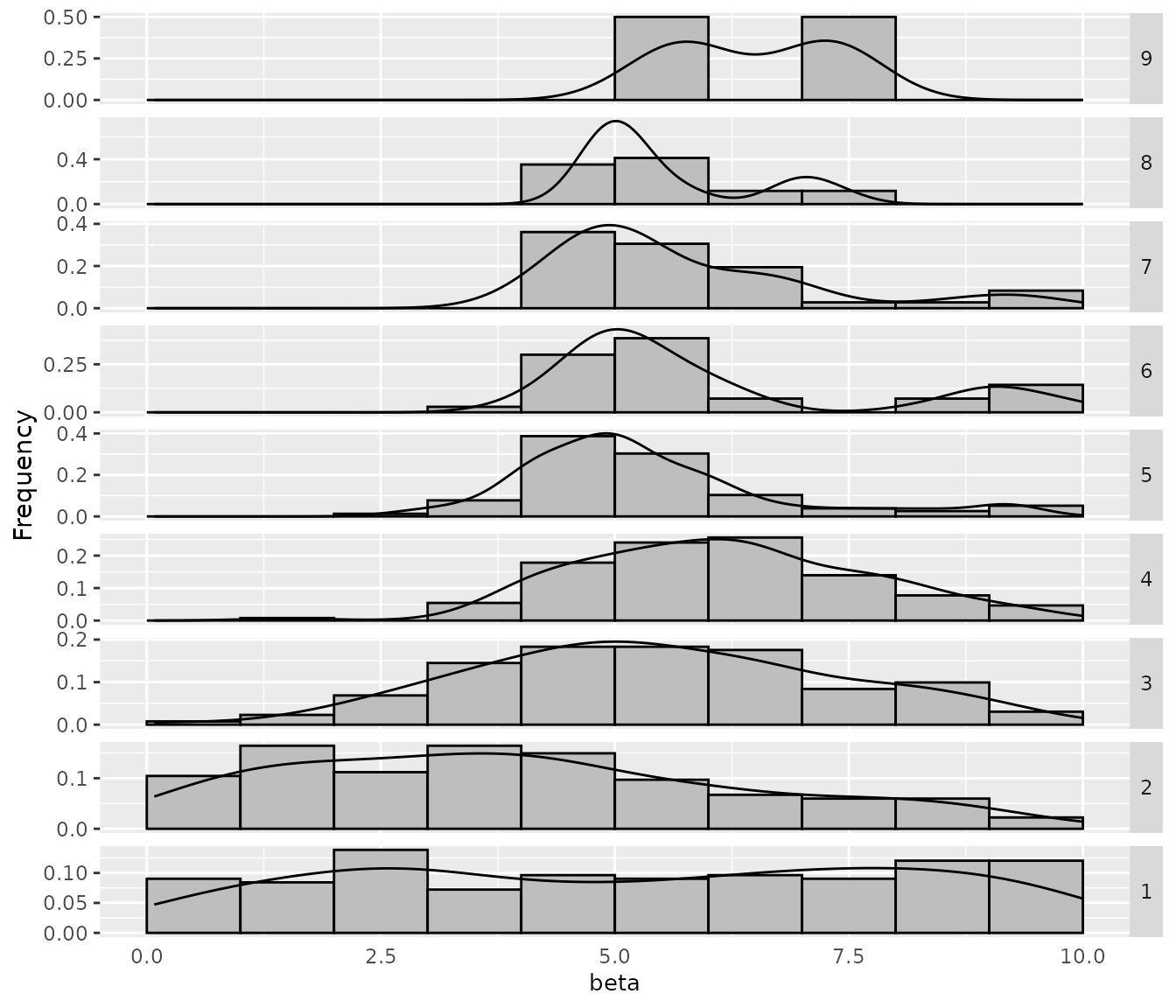
If you would like to see more details, a plot showing the sampling by iteration can be obtained with thesampling_frequency_iterationfunction. This plot shows the convergence of the configuration process reflected in the parameter values sampled each iteration:
In some cases, you may want to assess how the sampling frequencies of two parameters are related. You can visualize the joint sampling frequency of two parameters using the sampling_heatmapfunction. By default, this plot uses the elite configurations values (of all configurations), you can allow the plot to show all sampled configurations using the only_elite argument. You must select two parameters using the param_names argument, for example:
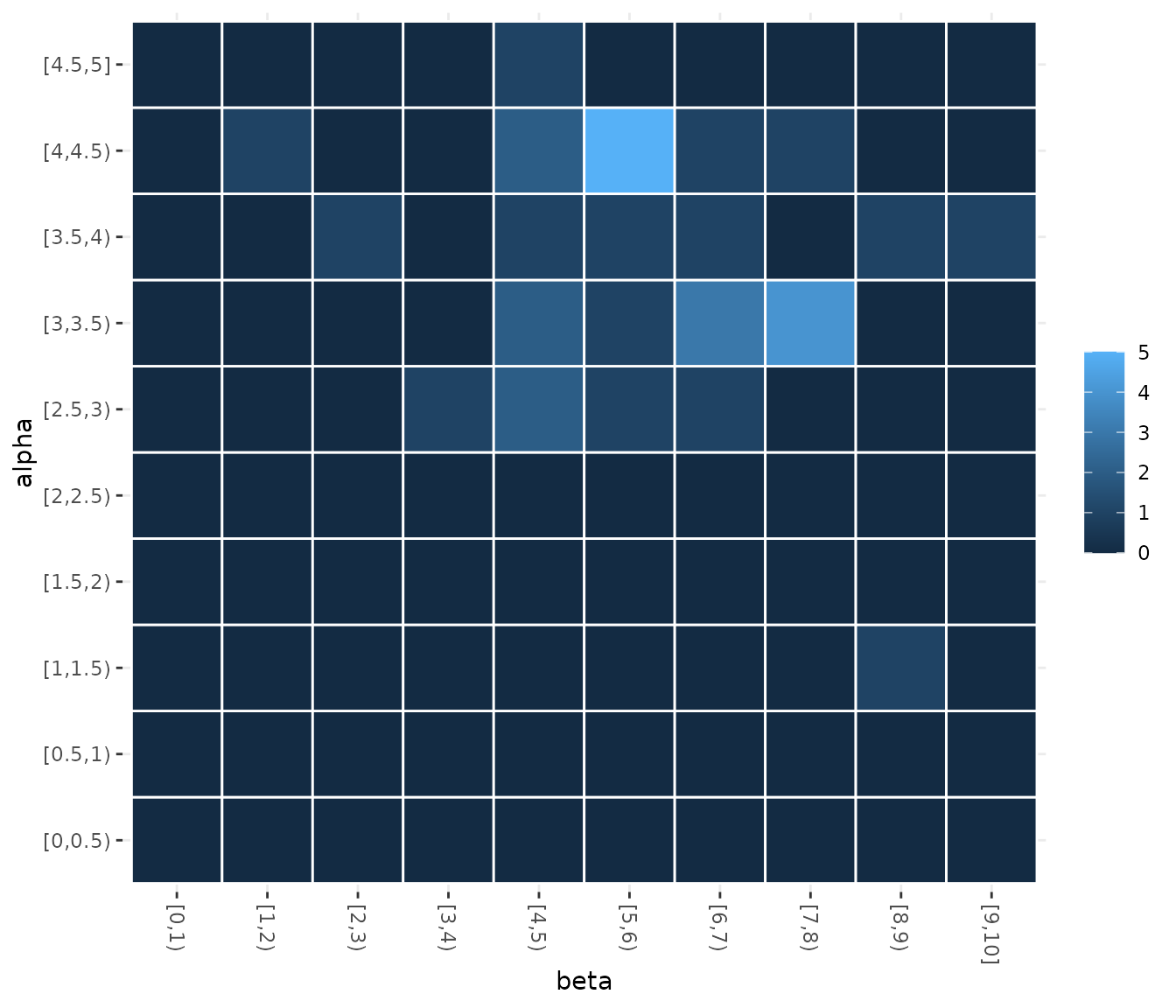
You can also select the iterations from which configurations will be selected using the iterations argument. The size of the intervals considered for numerical parameters in the heatmap can be also adjusted, see the example to have more details.
If you would like to display a set of configurations directly provided by you, use the sampling_heatmap2 function. In both sampling_heatmap2 and sampling_heatmap2, you can adjust the number of intervals to be displayed for numerical parameters using the sizes argument. For example, we set to 5 the number of intervals displayed for the second parameter, which is numerical, using sizes=c(0,5). The the 0 value in this argument indicates that the default interval size should be used. In this case, we set 0 for the first parameter but note that it is not possible to adjust the number of intervals for categorical or ordered parameter types.
sampling_heatmap2(iraceResults$allConfigurations, iraceResults$scenario$parameters,
                  param_names = c("localsearch","nnls"), sizes=c(0,5))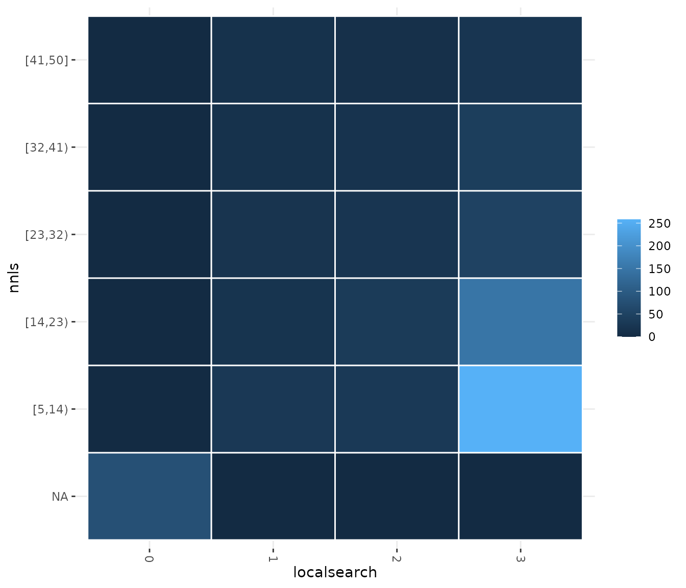
Sampling distance
You may like to have a general overview of the distance of the configurations sampled across the configuration process. This can allow you to assess the convergence of the configuration process. The mean distance between the sampled configurations can be visualized using thesampling_distance function. This function compares the parameter values of all configurations and aggregates these comparisons to calculate the overall distance:
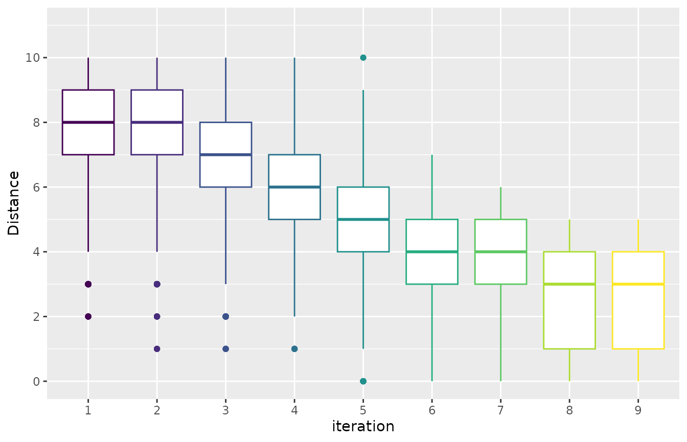
Note that for categorical and ordered parameters the comparison is straightforward, but this is not the case for numerical parameters. The argument t defines a percentage used to define a domain interval to assess equality of numerical parameters. For example, if the domain of a parameter is [0,10] and t=0.1 then when comparing any value to v=2 we define an intervals=t* (upper_bound -lower_bound) = 0.1*(10-0)=1. Then all values in the interval [v-s, v+s] [1,3] will be equal tov=2.