Evaluation of Dataset Alignment (original) (raw)
Introduction
In the realm of single-cell genomics, the ability to compare and integrate data across different conditions, datasets, or methodologies is crucial for deriving meaningful biological insights. This vignette introduces several functions designed to facilitate such comparisons and analyses by providing robust tools for evaluating and visualizing similarities and differences in high-dimensional data.
Functions for Evaluation of Dataset Alignment
comparecca: This function enables the comparison of datasets by applying Canonical Correlation Analysis (CCA). It helps assess how well two datasets align with each other, providing insights into the relationship between different single-cell experiments or conditions.comparepca: This function allows you to compare datasets using Principal Component Analysis (PCA). It evaluates how similar or different the principal components are between two datasets, offering a way to understand the underlying structure and variance in your data.comparepcasubspace: Extending the comparison to specific subspaces, this function focuses on subsets of principal components. It provides a detailed analysis of how subspace structures differ or align between datasets, which is valuable for fine-grained comparative studies.plotPairwiseDistancesDensity: To visualize the distribution of distances between pairs of samples, this function generates density plots. It helps in understanding the variation and relationships between samples in high-dimensional spaces.plotWassersteinDistance: This function visualizes the Wasserstein distance, a metric for comparing distributions, across datasets. It provides an intuitive view of how distributions differ between datasets, aiding in the evaluation of alignment and discrepancies.
Marker Gene Alignment
calculateHVGOverlap: To assess the similarity between datasets based on highly variable genes, this function computes the overlap coefficient. It measures how well the sets of highly variable genes from different datasets correspond to each other.calculateVarImpOverlap: Using Random Forest, this function identifies and compares the importance of genes for differentiating cell types between datasets. It highlights which genes are most critical in each dataset and compares their importance, providing insights into shared and unique markers.
Purpose and Applications
These functions collectively offer a comprehensive toolkit for comparing and analyzing single-cell data. Whether you are assessing alignment between datasets, visualizing distance distributions, or identifying key genes, these tools are designed to enhance your ability to derive meaningful insights from complex, high-dimensional data.
In this vignette, we will guide you through the practical use of each function, demonstrate how to interpret their outputs, and show how they can be integrated into your single-cell genomics workflow.
Preliminaries
In the context of the scDiagnostics package, this vignette demonstrates how to leverage various functions to evaluate and compare single-cell data across two distinct datasets:
reference_data: This dataset features meticulously curated cell type annotations assigned by experts. It serves as a robust benchmark for evaluating the accuracy and consistency of cell type annotations across different datasets, offering a reliable standard against which other annotations can be assessed.query_data: This dataset contains cell type annotations from both expert assessments and those generated using theSingleRpackage. By comparing these annotations with those from the reference dataset, you can identify discrepancies between manual and automated results, highlighting potential inconsistencies or areas requiring further investigation.
Some functions in the vignette are designed to work withSingleCellExperiment objects that contain data from only one cell type. We will create separate SingleCellExperimentobjects that only CD4 cells, to ensure compatibility with these functions.
# Load library
library(scran)
library(scater)

# Subset to CD4 cells
ref_data_cd4 <- reference_data[, which(reference_data$expert_annotation == "CD4")]
query_data_cd4 <- query_data_cd4 <- query_data[, which(query_data$expert_annotation == "CD4")]

# Select highly variable genes
ref_top_genes <- getTopHVGs(ref_data_cd4, n = 500)
query_top_genes <- getTopHVGs(query_data_cd4, n = 500)
common_genes <- intersect(ref_top_genes, query_top_genes)

# Subset data by common genes
ref_data_cd4 <- ref_data_cd4[common_genes,]
query_data_cd4 <- query_data_cd4[common_genes,]

# Run PCA on both datasets
ref_data_cd4 <- runPCA(ref_data_cd4)
query_data_cd4 <- runPCA(query_data_cd4)
compareCCA
The compareCCA function evaluates how well cell types from the query dataset align with those from the reference dataset using Canonical Correlation Analysis (CCA). It’s particularly useful for annotating cells in the query dataset based on their similarity to the reference data.
compareCCA performs the following steps:
- CCA Computation: It computes the canonical correlation between the query and reference datasets. CCA identifies pairs of canonical variables that maximize the correlation between the datasets.
- Correlation Analysis: The function then calculates the correlation between canonical variables of the query and reference datasets to determine how well they match.
- Annotation Assignment: Based on the highest correlations, the function assigns the most similar reference cell type to each query cell. This helps in transferring annotations from the reference dataset to the query dataset.
# Perform CCA
cca_comparison <- compareCCA(query_data = query_data_cd4,
                             reference_data = ref_data_cd4,
                             query_cell_type_col = "expert_annotation",
                             ref_cell_type_col = "expert_annotation",
                             pc_subset = 1:5)
plot(cca_comparison)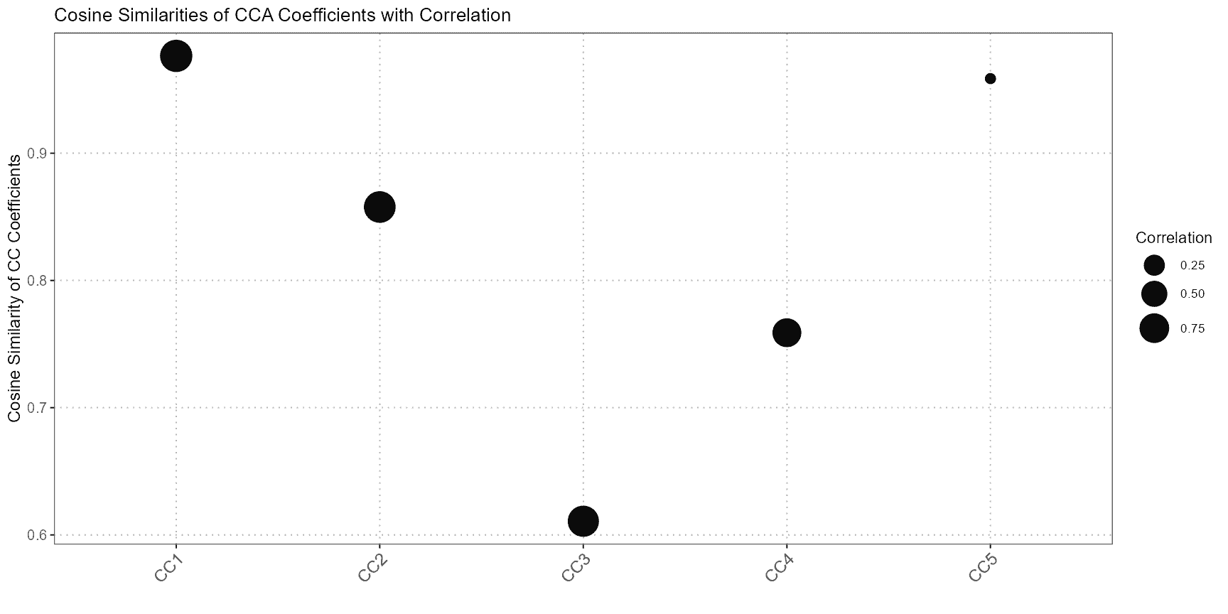
comparePCA
The comparePCA function compares the PCA subspaces between the query and reference datasets. It calculates the principal angles between the PCA subspaces to assess the alignment and similarity between them. This is useful for understanding how well the dimensionality reduction spaces of your datasets match.
comparePCA operates as follows:
- PCA Computation: It computes PCA for both query and reference datasets, reducing them into lower-dimensional spaces.
- Subspace Comparison: The function calculates the principal angles between the PCA subspaces of the query and reference datasets. These angles help determine how closely the subspaces align.
- Distance Metrics: It uses distance metrics based on principal angles to quantify the similarity between the datasets.
# Perform PCA
pca_comparison <- comparePCA(query_data = query_data_cd4,
                             reference_data = ref_data_cd4,
                             query_cell_type_col = "expert_annotation",
                             ref_cell_type_col = "expert_annotation",
                             pc_subset = 1:5,
                             metric = "cosine")
plot(pca_comparison)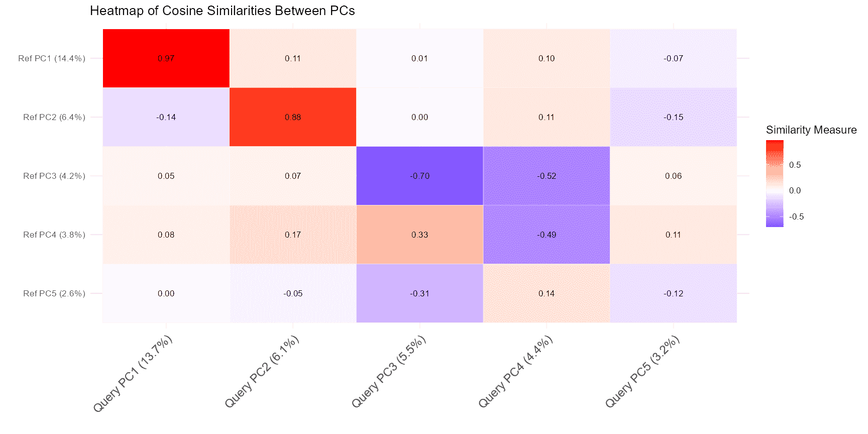
comparePCASubspace
In single-cell RNA-seq analysis, it is essential to assess the similarity between the subspaces spanned by the top principal components (PCs) of query and reference datasets. This is particularly important when comparing the structure and variation captured by each dataset. ThecomparePCASubspace function is designed to provide insights into how well the subspaces align by computing the cosine similarity between the loadings of the top variables for each PC. This analysis helps in determining the degree of correspondence between the datasets, which is critical for accurate cell type annotation and data integration.
comparePCASubspace performs the following operations:
- Cosine Similarity Calculation: The function computes the cosine similarity between the loadings of the top variables for each PC in both the query and reference datasets. This similarity measures how closely the two datasets align in the space spanned by their principal components.
- Selection of Top Similarities: The function selects the top cosine similarity scores and stores the corresponding PC indices from both datasets. This step identifies the most aligned principal components between the two datasets.
- Variance Explained Calculation: It then calculates the average percentage of variance explained by the selected top PCs. This helps in understanding how much of the data’s variance is captured by these components.
- Weighted Cosine Similarity Score: Finally, the function computes a weighted cosine similarity score based on the top cosine similarities and the average percentage of variance explained. This score provides an overall measure of subspace alignment between the datasets.
# Compare PCA subspaces between query and reference data
subspace_comparison <- comparePCASubspace(query_data = query_data_cd4,
                                          reference_data = ref_data_cd4,
                                          query_cell_type_col = "expert_annotation",
                                          ref_cell_type_col = "expert_annotation",
                                          pc_subset = 1:5)

# View weighted cosine similarity score
subspace_comparison$weighted_cosine_similarity
#> [1] 0.2462199
# Plot output for PCA subspace comparison (if a plot method is available)
plot(subspace_comparison)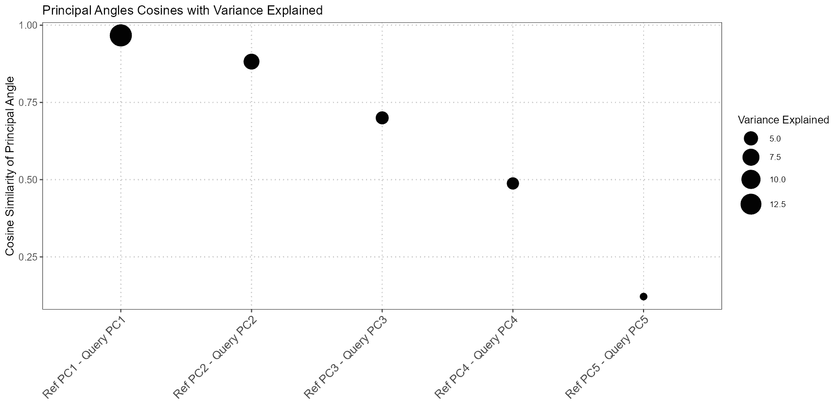
In the results:
- Cosine Similarity: The values in principal_angles_cosines indicate the degree of alignment between the principal components of the query and reference datasets. Higher values suggest stronger alignment.
- Variance Explained: The average_variance_explained vector provides the average percentage of variance captured by the selected top PCs in both datasets. This helps assess the importance of these PCs in explaining data variation.
- Weighted Cosine Similarity: The weighted_cosine_similarity score combines the cosine similarity with variance explained to give a comprehensive measure of how well the subspaces align. A higher score indicates that the datasets are well-aligned in the PCA space.
By using comparePCASubspace, you can quantify the alignment of PCA subspaces between query and reference datasets, aiding in the evaluation of dataset integration and the reliability of cell type annotations.
plotPairwiseDistancesDensity
Purpose
The plotPairwiseDistancesDensity function is designed to calculate and visualize the pairwise distances or correlations between cell types in query and reference datasets. This function is particularly useful in single-cell RNA sequencing (scRNA-seq) analysis, where it is essential to evaluate the consistency and reliability of cell type annotations by comparing their expression profiles.
Functionality
The function operates on SingleCellExperiment objects, which are commonly used to store single-cell data, including expression matrices and associated metadata. Users specify the cell types of interest in both the query and reference datasets, and the function computes either the distances or correlation coefficients between these cells.
When principal component analysis (PCA) is applied, the function projects the expression data into a lower-dimensional PCA space, which can be specified by the user. This allows for a more focused analysis of the major sources of variation in the data. Alternatively, if no dimensionality reduction is desired, the function can directly use the expression data for computation.
Depending on the user’s choice, the function can calculate pairwise Euclidean distances or correlation coefficients. The resulting values are used to compare the relationships between cells within the same dataset (either query or reference) and between cells across the two datasets.
Interpretation
The output of the function is a density plot generated by ggplot2, which displays the distribution of pairwise distances or correlations. The plot provides three key comparisons:
- Query vs. Query,
- Reference vs. Reference,
- Query vs. Reference.
By examining these density curves, users can assess the similarity of cells within each dataset and across datasets. For example, a higher density of lower distances in the “Query vs. Reference” comparison would suggest that the query and reference cells are similar in their expression profiles, indicating consistency in the annotation of the cell type across the datasets.
This visual approach offers an intuitive way to diagnose potential discrepancies in cell type annotations, identify outliers, or confirm the reliability of the cell type assignments.
# Example usage of the function
plotPairwiseDistancesDensity(query_data = query_data,
reference_data = reference_data,
query_cell_type_col = "expert_annotation",
ref_cell_type_col = "expert_annotation",
cell_type_query = "CD4",
cell_type_ref = "CD4",
pc_subset = 1:5,
distance_metric = "euclidean",
correlation_method = "spearman")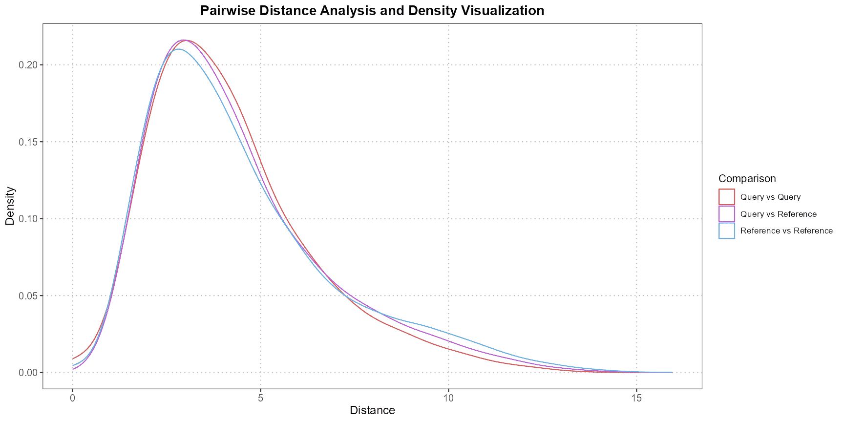 This example demonstrates how to compare CD4 cells between a query and reference dataset, with PCA applied to the first five principal components and pairwise Euclidean distances calculated. The output is a density plot that helps visualize the distribution of these distances, aiding in the interpretation of the similarity between the two datasets.
plotWassersteinDistance
The plotWassersteinDistance function creates a density plot to compare the Wasserstein distances between a reference dataset and a query dataset under the null hypothesis. The null hypothesis assumes that both datasets are drawn from the same distribution. This function is useful for evaluating how different the query data is from the reference data based on their Wasserstein distances.
How the Function Operates
- Projecting Data into PCA Space:
- The query data is projected into the PCA space defined by the reference data. This step aligns the datasets by reducing their dimensions using principal components.
- Calculating the Null Distribution:
- The function generates a null distribution of Wasserstein distances by repeatedly sampling subsets from the reference data. This represents the distribution of distances you would expect if both datasets were from the same source.
- Computing Reference-Query Distance:
- The Wasserstein distance between the projected reference and query data is computed. This distance quantifies how different the query dataset is from the reference dataset.
- Creating the Density Plot:
- The function generates a density plot of the null distribution of Wasserstein distances.
- Vertical lines are added to indicate:
- The significance threshold: Distances greater than this threshold suggest a significant difference between the datasets.
- The reference-query distance: The actual distance between the reference and query datasets.
Interpretation
- Density Plot: This plot shows the distribution of Wasserstein distances under the assumption that the datasets are similar.
- Significance Threshold Line: If the reference-query distance exceeds this line, it indicates a significant difference between the datasets.
- Reference-Query Distance Line: This line shows the observed distance between the reference and query datasets. If this line is to the right of the significance threshold, the difference is statistically significant.
Code Example
# Generate the Wasserstein distance density plot
plotWassersteinDistance(query_data = query_data_cd4,
                        reference_data = ref_data_cd4,
                        query_cell_type_col = "expert_annotation",
                        ref_cell_type_col = "expert_annotation",
                        pc_subset = 1:5,
                        alpha = 0.05)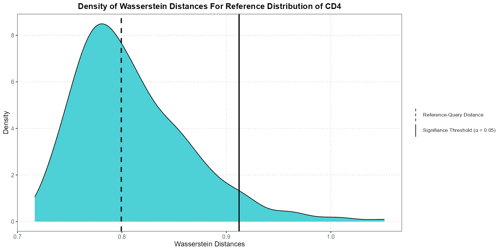
This example demonstrates how to use theplotWassersteinDistance function to compare Wasserstein distances between CD4 cells in the reference and query datasets. The resulting plot helps determine whether the difference between the datasets is statistically significant.
Marker Gene Alignment
calculateHVGOverlap
The calculateHVGOverlap function computes the overlap coefficient between two sets of highly variable genes (HVGs) from a reference dataset and a query dataset. The overlap coefficient is a measure of similarity between the two sets, reflecting how much the HVGs in one dataset overlap with those in the other.
How the Function Operates
The function begins by ensuring that the input vectorsreference_genes and query_genes are character vectors and that neither of them is empty. Once these checks are complete, the function identifies the common genes between the two sets using the intersect function, which finds the intersection of the two gene sets.
Next, the function calculates the size of this intersection, representing the number of genes common to both sets. The overlap coefficient is then computed by dividing the size of the intersection by the size of the smaller set of genes. This ensures that the coefficient is a value between 0 and 1, where 0 indicates no overlap and 1 indicates complete overlap.
Finally, the function rounds the overlap coefficient to two decimal places before returning it as the output.
Interpretation
The overlap coefficient quantifies the extent to which the HVGs in the reference dataset align with those in the query dataset. A higher coefficient indicates a stronger similarity between the two datasets in terms of their HVGs, which can suggest that the datasets are more comparable or that they capture similar biological variability. Conversely, a lower coefficient indicates less overlap, suggesting that the datasets may be capturing different biological signals or that they are less comparable.
Code Example
# Load library to get top HVGs
library(scran)

# Select the top 500 highly variable genes from both datasets
ref_var_genes <- getTopHVGs(reference_data, n = 500)
query_var_genes <- getTopHVGs(query_data, n = 500)

# Calculate the overlap coefficient between the reference and query HVGs
overlap_coefficient <- calculateHVGOverlap(reference_genes = ref_var_genes,
                                           query_genes = query_var_genes)

# Display the overlap coefficient
overlap_coefficient
#> [1] 0.96
calculateVarImpOverlap
Overview
The calculateVarImpOverlap function helps you identify and compare the most important genes for distinguishing cell types in both a reference dataset and a query dataset. It does this using the Random Forest algorithm, which calculates how important each gene is in differentiating between cell types.
Usage
To use the function, you need to provide a reference dataset containing expression data and cell type annotations. Optionally, you can also provide a query dataset if you want to compare gene importance across both datasets. The function allows you to specify which cell types to analyze and how many trees to use in the Random Forest model. Additionally, you can decide how many top genes you want to compare between the datasets.
Code Example
Let’s say you have a reference dataset (reference_data) and a query dataset (query_data). Both datasets contain expression data and cell type annotations, stored in columns named “expert_annotation” and “SingleR_annotation”, respectively. You want to calculate the importance of genes using 500 trees and compare the top 50 genes between the datasets.
Here’s how you would use the function:
# RF function to compare (between datasets) which genes are best at differentiating cell types
rf_output <- calculateVarImpOverlap(reference_data = reference_data,
                                    query_data = query_data,
                                    query_cell_type_col = "expert_annotation",
                                    ref_cell_type_col = "expert_annotation",
                                    n_tree = 500,
                                    n_top = 50)

# Comparison table
rf_output$var_imp_comparison
#>     B_and_plasma-CD4     B_and_plasma-CD8 B_and_plasma-Myeloid
#>                 0.84                 0.90                 0.80
#>              CD4-CD8          CD4-Myeloid          CD8-Myeloid
#>                 0.80                 0.90                 0.84
Interpretation:
After running the function, you’ll receive the importance scores of genes for each pair of cell types in your reference dataset. If you provided a query dataset, you’ll also get the importance scores for those cell types. The function will tell you how much the top genes in the reference and query datasets overlap, which helps you understand if the same genes are important for distinguishing cell types across different datasets.
For example, if there’s a high overlap, it suggests that similar genes are crucial in both datasets for differentiating the cell types, which could be important for validating your findings or identifying robust markers.
Conclusion
In this vignette, we have demonstrated a comprehensive suite of functions designed to enhance the analysis and comparison of single-cell genomics datasets. compareCCA and comparePCAfacilitate the evaluation of dataset alignment through canonical correlation analysis and principal component analysis, respectively. These tools help in assessing the correspondence between datasets and identifying potential batch effects or differences in data structure.comparePCASubspace further refines this analysis by focusing on specific subspaces within the PCA space, providing a more granular view of dataset similarities.
plotPairwiseDistancesDensity andplotWassersteinDistance offer advanced visualization techniques for comparing distances and distributions across datasets. These functions are crucial for understanding the variability and overlap between datasets in a more intuitive and interpretable manner. On the other hand, calculateHVGOverlap andcalculateVarImpOverlap provide insights into gene variability and importance, respectively, by comparing highly variable genes and variable importance scores across reference and query datasets.
Together, these functions form a robust toolkit for single-cell genomics analysis, enabling researchers to conduct detailed comparisons, visualize data differences, and validate the relevance of their findings across different datasets. Incorporating these tools into your research workflow will help ensure more accurate and insightful interpretations of single-cell data, ultimately advancing the understanding of cellular processes and improving experimental outcomes.
R Session Info
R version 4.4.0 (2024-04-24 ucrt)
Platform: x86_64-w64-mingw32/x64
Running under: Windows 11 x64 (build 22631)

Matrix products: default


locale:
[1] LC_COLLATE=English_United States.utf8
[2] LC_CTYPE=English_United States.utf8
[3] LC_MONETARY=English_United States.utf8
[4] LC_NUMERIC=C
[5] LC_TIME=English_United States.utf8

time zone: America/New_York
tzcode source: internal

attached base packages:
[1] stats4    stats     graphics  grDevices utils     datasets  methods
[8] base

other attached packages:
 [1] scater_1.32.0               ggplot2_3.5.1
 [3] scran_1.32.0                scuttle_1.14.0
 [5] SingleCellExperiment_1.26.0 SummarizedExperiment_1.34.0
 [7] Biobase_2.64.0              GenomicRanges_1.56.0
 [9] GenomeInfoDb_1.40.1         IRanges_2.38.0
[11] S4Vectors_0.42.0            BiocGenerics_0.50.0
[13] MatrixGenerics_1.16.0       matrixStats_1.3.0
[15] scDiagnostics_0.99.6        BiocStyle_2.32.0

loaded via a namespace (and not attached):
 [1] gridExtra_2.3             rlang_1.1.3
 [3] magrittr_2.0.3            compiler_4.4.0
 [5] DelayedMatrixStats_1.26.0 systemfonts_1.1.0
 [7] vctrs_0.6.5               pkgconfig_2.0.3
 [9] crayon_1.5.2              fastmap_1.2.0
[11] XVector_0.44.0            labeling_0.4.3
[13] utf8_1.2.4                rmarkdown_2.27
[15] UCSC.utils_1.0.0          ggbeeswarm_0.7.2
[17] ragg_1.3.2                purrr_1.0.2
[19] xfun_0.44                 bluster_1.14.0
[21] zlibbioc_1.50.0           cachem_1.1.0
[23] beachmat_2.20.0           jsonlite_1.8.8
[25] highr_0.11                DelayedArray_0.30.1
[27] BiocParallel_1.38.0       irlba_2.3.5.1
[29] parallel_4.4.0            cluster_2.1.6
[31] R6_2.5.1                  bslib_0.7.0
[33] ranger_0.16.0             limma_3.60.2
[35] jquerylib_0.1.4           Rcpp_1.0.12
[37] bookdown_0.39             knitr_1.46
[39] Matrix_1.7-0              igraph_2.0.3
[41] tidyselect_1.2.1          rstudioapi_0.16.0
[43] abind_1.4-5               yaml_2.3.8
[45] viridis_0.6.5             codetools_0.2-20
[47] lattice_0.22-6            tibble_3.2.1
[49] withr_3.0.0               evaluate_0.23
[51] desc_1.4.3                pillar_1.9.0
[53] BiocManager_1.30.23       generics_0.1.3
[55] sparseMatrixStats_1.16.0  munsell_0.5.1
[57] scales_1.3.0              glue_1.7.0
[59] metapod_1.12.0            tools_4.4.0
[61] data.table_1.15.4         BiocNeighbors_1.22.0
[63] ScaledMatrix_1.12.0       locfit_1.5-9.9
[65] fs_1.6.4                  grid_4.4.0
[67] edgeR_4.2.0               colorspace_2.1-0
[69] GenomeInfoDbData_1.2.12   beeswarm_0.4.0
[71] BiocSingular_1.20.0       vipor_0.4.7
[73] cli_3.6.2                 rsvd_1.0.5
[75] textshaping_0.4.0         fansi_1.0.6
[77] viridisLite_0.4.2         S4Arrays_1.4.1
[79] dplyr_1.1.4               gtable_0.3.5
[81] sass_0.4.9                digest_0.6.35
[83] SparseArray_1.4.8         ggrepel_0.9.5
[85] dqrng_0.4.1               farver_2.1.2
[87] htmlwidgets_1.6.4         memoise_2.0.1
[89] htmltools_0.5.8.1         pkgdown_2.0.9
[91] lifecycle_1.0.4           httr_1.4.7
[93] transport_0.15-2          statmod_1.5.0