Running AlexNet on Raspberry Pi with Compute Library (original) (raw)

If you’d like to develop your Convolutional Neural Networks using just the Compute Library and a Raspberry Pi, this step-by-step guide will show you how… and it comes complete with all the tools you’ll need to get up and running.

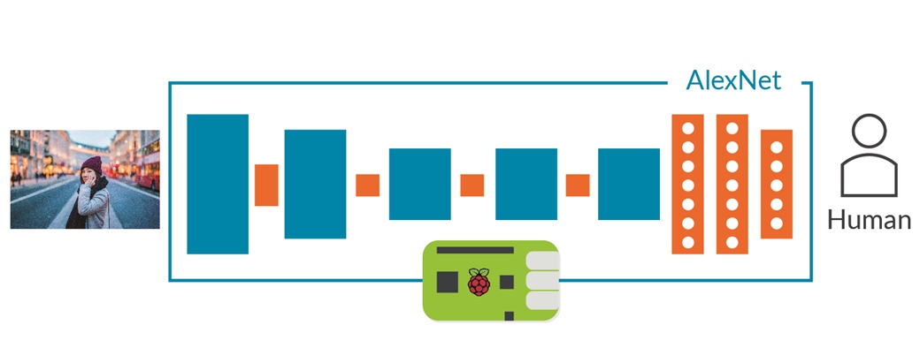
If you follow all the steps outlined here indeed, by the end of the post you’ll be up and running with one of the first Deep Convolutional Neural Networks (CNN) designed to recognize 1000 different objects: AlexNet!

Getting started

If you haven’t read my previous blog on how to apply a cartoon effect with the Compute Library, I’d suggest starting with that. It’s a simple example, but it will give you all the information you need to compile or cross-compile the library for Raspberry Pi.

In addition to some basic knowledge of the Compute Library, this tutorial assumes some knowledge of a CNN; you don’t need to be an expert, just have an idea of the main functions.

Everything else can be found in the following .7z file, which contains:

1. The AlexNet model (the same one as in the Caffe Model Zoo)
2. A text file, containing the ImageNet labels required to map the predicted objects to the name of the classes
3. Several images in ppm file format ready to be used with the network

Please download the required files to your host machine (Debian based) or to your Raspberry Pi:

compute_library_alexnet files

Within the folder "alexnet_tutorial" you should have everything for this tutorial.

The requirements for your Raspberry Pi and host machine are:

1. Raspberry Pi 2 or 3 with Ubuntu Mate 16.04.02
2. A blank Micro SD card: we highly recommend a Class 6 or Class 10 microSDHC card with 8 GB (minimum 6GB)
3. Router + Ethernet cable

A word about the Graph API

In release 17.09 of the Compute Library, we introduced an important feature to make life easier for developers, and anyone else benchmarking the library: the graph API.

The graph API’s primary function is to reduce the boilerplate code, but it can also reduce errors in your code and improve its readability. It’s simple and easy-to-use, with a stream interface that’s designed to be similar to other C++ objects.

At the current stage, the graph API only supports the ML functions (i.e. convolution, fully connected, activation, pooling...) and can only be used if the library has been compiled with both NEON and OpenCL enabled (neon=1 and opencl=1).

Note: if your platform doesn't have OpenCL don't worry (i.e. Raspberry Pi), the Graph API will automatically fall back onto using NEON, however you do need to compile the Compute Library with both NEON and OpenCL enabled.

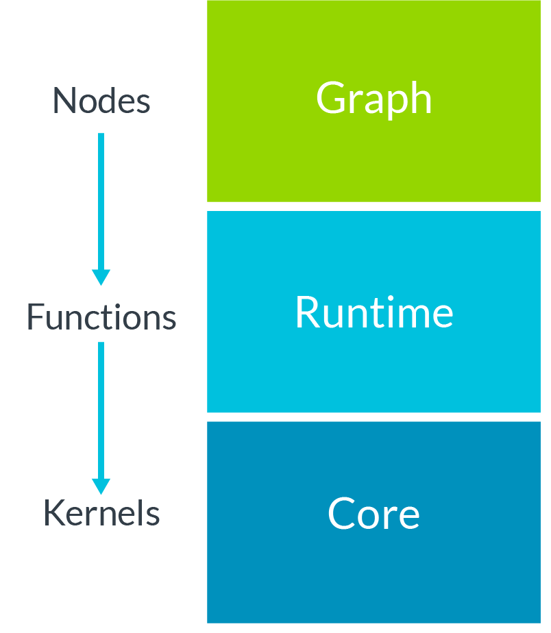
In terms of building blocks, the graph API represents the third computation block, together with core and runtime. In terms of hierarchy, the graph API lies just above the runtime, which in turn lies above the core block.

Introducing AlexNet

In 2012, AlexNet shot to fame when it won the ImageNet Large Scale Visual Recognition Challenge (ILSVRC), an annual challenge that aims to evaluate algorithms for object detection and image classification.

The ILSVRC evaluates the success of image classification solutions is using two important metrics: the top-5 and top-1 errors. Given a set of N images (usually called “test images”) and mapped a target class for each one:

• top-1 error checks if the top predicted class is the same as the target class
• top-5 error checks if the target class is one of the top five predictions

For both, the top error is calculated as, "the number of times the predicted class does not match the target class, divided by the total number of test images". In other words, a lower score is better.

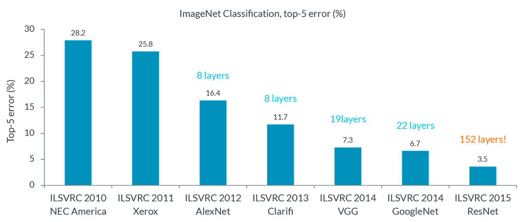
The authors of AlexNet – Alex Krizhevsky, Geoffrey Hinton, and Ilya Sutskever of the SuperVision group – achieved a top-5 error around 16%, which was a staggeringly good result back in 2012. To put it into context, until that year no one had been able to go under 20%. AlexNet was also more than 10% better than the runner up.

After 2012, more accurate and deeper CNNs began to proliferate, as the graph below shows

What are the ingredients of AlexNet?

AlexNet is made up of eight trainable layers: five convolution layers and three fully connected layers. All the trainable layers are followed by a ReLu activation function, except for the last fully connected layer, where the Softmax function is used.

Besides the trainable layers, the network also has:

1. Three pooling layers
2. Two normalization layers
3. One dropout layer (only used for training to reduce the overfitting)

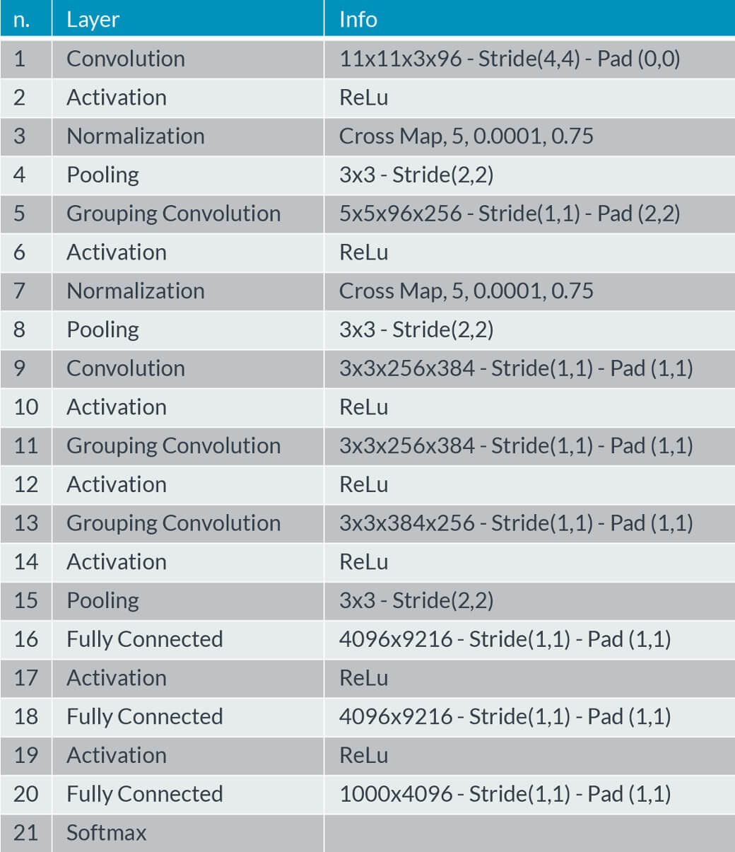
Grouping

If you look at the table above, you’ll notice that some convolution layers are actually ‘grouping convolutions’ – an efficient engineering trick that allows the acceleration of the network over two GPUs, without sacrificing accuracy.

If the group size is set to two, the first half of the filters will be connected just to the first half of the input feature maps; the second half will connect to the second half.

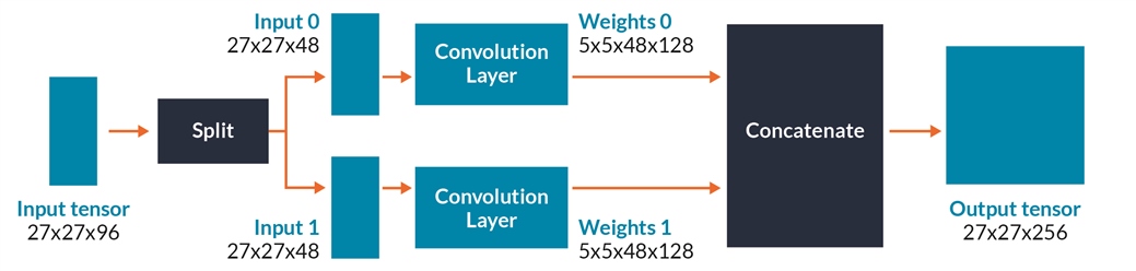
The grouping convolution not only allows you to spread the workload over multiple GPUs, it also reduces the number of MACs needed for the layer by half

A closer look at the code: examples/graph_alexnet.cpp

A C++ implementation of AlexNet using the graph API is proposed in examples/graph_alexnet.cpp.

To run the AlexNet example we need four command line arguments:

./graph_alexnet

Where:

1. is the the type of acceleration (NEON=0 or OpenCL=1)
2. <cnn_data>: Path to cnn_data
3. <input_image>: Path to your input image (only ppm files are supported)
4. : Path to your ImageNet labels

With the following sections I am going to describe the key aspects of this example.

Header files

In order to use the graph API we need to include three header files:

// Contains the definitions for the graph #include "arm_compute/graph/Graph.h"

// Contains the definitions for the nodes (convolution, pooling, fully connected) #include "arm_compute/graph/Nodes.h"

// Contains the utility functions for the graph such as the accessors for the input, trainable and output nodes. The accessors will be presented when we are going to talk about the graph. #include "utils/GraphUtils.h"

Mean subtraction pre-processing

A pre-processing stage is needed for preparing the input RGB image before feeding the network, so we’re going to subtract the channel means from each individual colour channel. This operation will centre the red, green and blue channels around the origin.

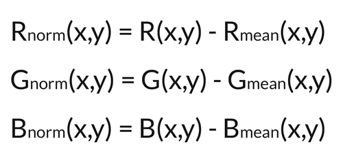
Where:

• r_norm(x,y), g_norm(x,y), b_norm(x,y) are the RGB values at coordinates x,y after the mean subtraction
• r(x,y), g(x,y), b(x,y) are the RGB values at coordinates x,y before the mean subtraction
• r_mean, g_mean and b_mean are the mean values to use for the RGB channels

For simplicity, we’ve already hard-coded the mean values to use in the example:

constexpr float mean_r = 122.68f; /* Mean value to subtract from red channel / constexpr float mean_g = 116.67f; / Mean value to subtract from green channel / constexpr float mean_b = 104.01f; / Mean value to subtract from blue channel */

If you’ve not heard of mean subtraction pre-processing before, have a look at the Compute Image Mean section on the Caffe website

Network description

The body of the network is described through the graph API.

The graph consists of three main parts:

1. MANDATORY: one input "Tensor object". This layer describes the geometry of the input data along with the data type to use. In this case, we’ll have a 3D input image with shape 227x227x3, using the FP32 data type
2. The Convolution Neural Network layers – or ‘nodes’ in the graph's terminology – needed for the network
3. MANDATORY: one output "Tensor object", used to get the result back from the network

As you will notice from the example, the Tensor objects (input and output) and all the trainable layers accept an input function called "accessor".

The accessor is the only way to access the internal Tensors.

• The accessor used by the input Tensor object can initialize the input Tensor of the network. This function can also be responsible for the mean subtraction pre-processing and reading the input image from a file or camera
• The accessor used by the trainable layers (i.e. convolution, fully connected, etc) can initialize the weights and the biases reading – e.g. the values from a numpy file
• The accessor used by the output Tensor object can return the result of the classification, along with the score

If you are curious to know how the accessor works, take a look at utils GraphUtils.h where you can find a few ready-to-use accessors for your Tensor objects and trainable layers.

Time to classify!

Now it is time to turn on your Raspberry Pi and test AlexNet with the same images.

Note: the following steps assume you are in the home directory of your Raspberry Pi or host machine.

On your Raspberry Pi enter the following commands

Install unzip

sudo apt-get install unzip

Download the zip file with the AlexNet model, input images and labels

wget

Create a new folder

mkdir assets_alexnet

Unzip

unzip compute_library_alexnet.zip -d assets_alexnet

If you are compiling natively on your Raspberry Pi, use the following instructions. If you’re cross-compiling, see the appropriate section below.

On your Raspberry Pi:

Clone Compute Library

git clone https://github.com/Arm-software/ComputeLibrary.git

Enter ComputeLibrary folder

cd ComputeLibrary

Native build the library and the examples

scons Werror=1 debug=0 asserts=0 neon=1 opencl=1 examples=1 build=native –j2

Once the library has been compiled where are ready to classify our go-kart!

export LD_LIBRARY_PATH=build/

PATH_ASSETS=../assets_alexnet

./build/examples/graph_alexnet 0 PATHASSETSPATH_ASSETS PATHA​SSETSPATH_ASSETS/go_kart.ppm $PATH_ASSETS/labels.txt

If you’re cross-compiling, on your host machine:

Clone Compute Library

git clone https://github.com/Arm-software/ComputeLibrary.git

Enter ComputeLibrary folder

cd ComputeLibrary

Build the library and the examples

scons Werror=1 debug=0 asserts=0 neon=1 opencl=1 examples=1 os=linux arch=armv7a -j4

Copy the example and dynamic libraries on the Raspberry Pi

scp build/example/graph_alexnet build/libarm_compute.so build/libarm_compute_core.so build/libarm_compute_graph.so @:Desktop

where:

• <username_raspberrypi>: username used on your Raspberry Pi
• <ip_addr_raspberrypi>: IP address of your Raspberry Pi

Open the SSH session from your host machine:

ssh @

Within the SSH session:

cd Desktop

export LD_LIBRARY_PATH=build/

PATH_ASSETS=../assets_alexnet

./build/examples/graph_alexnet 0 PATHASSETSPATH_ASSETS PATHA​SSETSPATH_ASSETS/go_kart.ppm $PATH_ASSETS/labels.txt

Whether or not you’re building the library natively, the output should look like this:

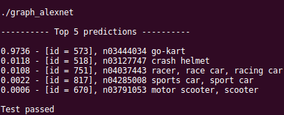
And that’s it!

Congratulations – you got there! I hope you had fun and, more importantly, I hope this will help you to develop even more exciting and performant intelligent vision solutions on Arm.

Ciao for now!

Gian Marco

To find this tutorial, and many other resources, visit the Machine Learning Developer Community.

• 
  • April 28, 2025
• 
  • April 8, 2025
• 
  • January 28, 2025