Finding optimal resolution of hierarchical hypotheses with treeclimbR (original) (raw)
Introduction
treeclimbR is a method for analyzing hierarchical trees of entities, such as phylogenies, at different levels of resolution. It proposes multiple candidates (corresponding to different aggregation levels) that capture the latent signal, and pinpoints branches or leaves that contain features of interest, in a data-driven way. One motivation for such a multi-level analysis is that the most highly resolved entities (e.g., individual species in a microbial context) may not be abundant enough to allow a potential abundance difference between conditions to be reliably detected. Aggregating abundances on a higher level in the tree can detect families of species that are closely related and that all change (possibly weakly but) concordantly. At the same time, blindly aggregating to a higher level across the whole tree may imply losing the ability to pinpoint specific species with a strong signal that may not be shared with their closest neighbors in the tree. Taken together, this motivates the development of a data-dependent aggregation approach, which is also allowed to aggregate different parts of the tree at different levels of resolution.
If you are using treeclimbR, please cite Huang et al. (2021), which also contains the theoretical justifications and more details of the method.
Installation
treeclimbR can be installed from Bioconductor using the following code:
It integrates seamlessly with theTreeSummarizedExperiment class, which allows observed data, feature and sample annotations, as well as a tree representing the hierarchical relationship among features (or samples) to be stored in the same object.
Preparation
This vignette outlines the main functionality oftreeclimbR, using simulated example data provided with the package. We start by loading the packages that will be needed in the analyses below.
Differential abundance (DA) analysis
The differential abundance (DA) workflow in treeclimbRis suitable in situations where we have observed abundances (often counts) of a set of entities in a set of samples, the entities can be represented as leaves of a given tree, and we are interested in finding entities (or groups of entities in the same subtree) whose abundance is associated with some sample phenotype (e.g., different between two conditions). For example, in Huang et al. (2021) we studied differences in the abundance of microbial species between babies born vaginally or via C-section. We also investigated differences in miRNA abundances between groups of mice receiving transaortic constriction or sham surgery, and cell type abundance differences between conditions at different clustering granularities. In all these cases, the entities are naturally represented as leaves in a tree (a phylogenetic tree in the first case, a tree where internal nodes represent miRNA duplexes, primary transcripts, and clusters of miRNAs for the second, and a clustering tree defined based on the average similarity between baseline high-resolution cell clusters for the third).
Load and visualize example data
In this vignette, we will work with a simulated data set with 30 samples (15 from each of two conditions) and 100 features. 18 of the features are differentially abundant between the two conditions; this information is stored in the Signal column of the object’srowData. The features represent leaves in a tree, and the data is stored in a TreeSummarizedExperiment object. Below, we first load the data and visualize the tree and the corresponding data.
## Read data
da_lse <- readRDS(system.file("extdata", "da_sim_100_30_18de.rds",
                              package = "treeclimbR"))
da_lse
#> class: TreeSummarizedExperiment
#> dim: 100 30
#> metadata(1): parentNodeForSignal
#> assays(1): counts
#> rownames(100): t8 t85 ... t45 t92
#> rowData names(1): Signal
#> colnames(30): A_1 A_2 ... B_29 B_30
#> colData names(1): group
#> reducedDimNames(0):
#> mainExpName: NULL
#> altExpNames(0):
#> rowLinks: a LinkDataFrame (100 rows)
#> rowTree: 1 phylo tree(s) (100 leaves)
#> colLinks: NULL
#> colTree: NULL

## Generate tree visualization where true signal leaves are colored orange
## ...Find internal nodes in the subtrees where all leaves are differentially
##    abundant. These will be colored orange.
nds <- joinNode(tree = rowTree(da_lse),
                node = rownames(da_lse)[rowData(da_lse)$Signal])
br <- unlist(findDescendant(tree = rowTree(da_lse), node = nds,
                            only.leaf = FALSE, self.include = TRUE))
df_color <- data.frame(node = showNode(tree = rowTree(da_lse),
                                       only.leaf = FALSE)) |>
    mutate(signal = ifelse(node %in% br, "yes", "no"))
## ...Generate tree
da_fig_tree <- ggtree(tr = rowTree(da_lse), layout = "rectangular",
                      branch.length = "none",
                      aes(color = signal)) %<+% df_color +
    scale_color_manual(values = c(no = "grey", yes = "orange"))
## ...Zoom into the subtree defined by a particular node. In this case, we
##    know that all true signal leaves were sampled from the subtree defined
##    by a particular node (stored in metadata(da_lse)$parentNodeForSignal).
da_fig_tree <- scaleClade(da_fig_tree,
                          node = metadata(da_lse)$parentNodeForSignal,
                          scale = 4)

## Extract count matrix and scale each row to [0, 1]
count <- assay(da_lse, "counts")
scale_count <- t(apply(count, 1, FUN = function(x) {
    xx <- x
    rx <- (max(xx) - min(xx))
    (xx - min(xx))/max(rx, 1)
}))
rownames(scale_count) <- rownames(count)
colnames(scale_count) <- colnames(count)

## Plot tree and heatmap of scaled counts
## ...Generate sample annotation
vv <- gsub(pattern = "_.*", "", colnames(count))
names(vv) <- colnames(scale_count)
anno_c <- structure(vv, names = vv)
TreeHeatmap(tree = rowTree(da_lse), tree_fig = da_fig_tree,
            hm_data = scale_count, legend_title_hm = "Scaled\ncount",
            column_split = vv, rel_width = 0.6,
            tree_hm_gap = 0.3,
            column_split_label = anno_c) +
    scale_fill_viridis_c(option = "B") +
    scale_y_continuous(expand = c(0, 10))
#> Scale for fill is already present.
#> Adding another scale for fill, which will replace the existing scale.
#> Scale for y is already present.
#> Adding another scale for y, which will replace the existing scale.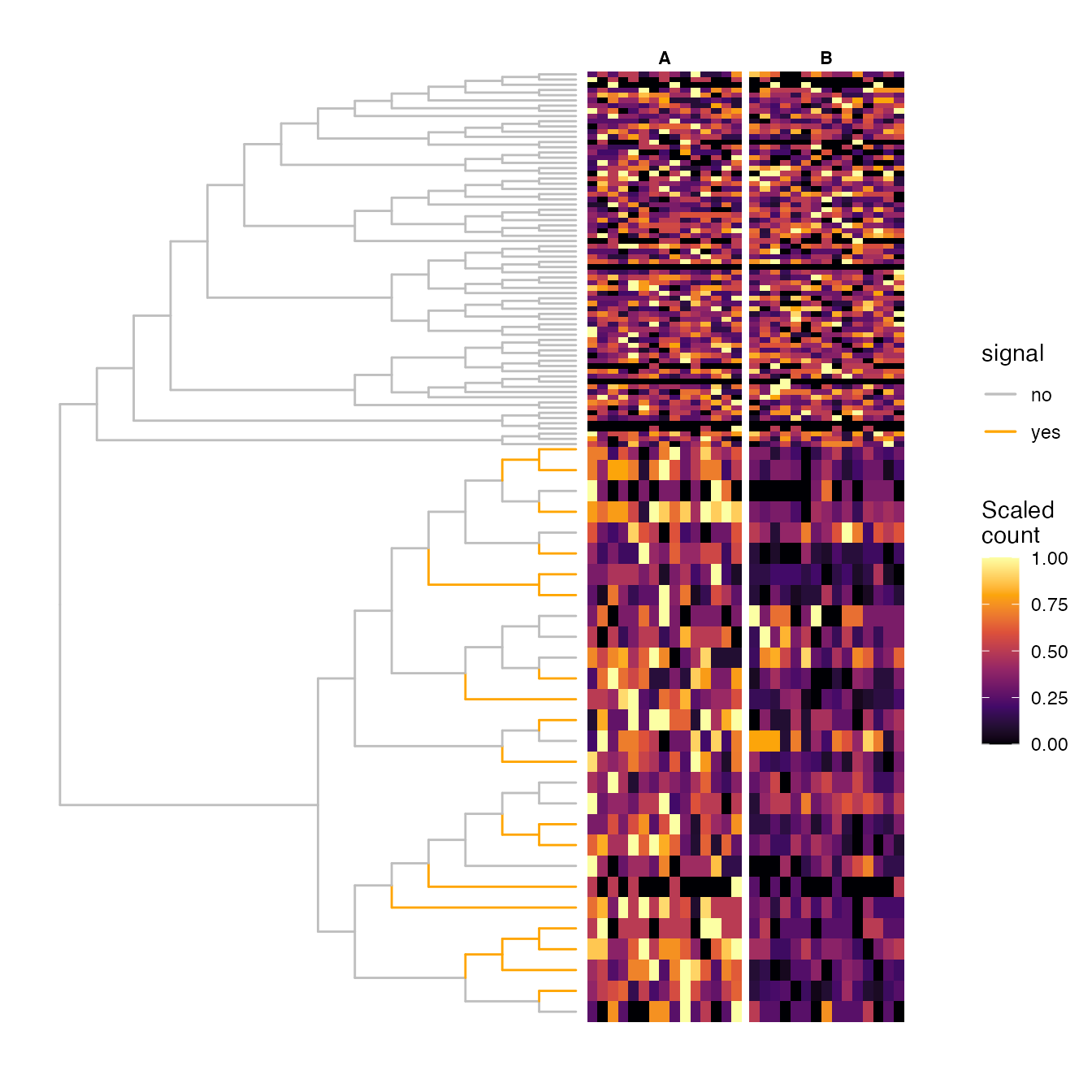
Aggregate counts for internal nodes
treeclimbR provides functionality to find an ‘optimal’ aggregation level at which to interpret hierarchically structured data. Starting from the TreeSummarizedExperiment above (containing the observed data as well as the tree for the features), the first step is to calculate aggregated values (in this case, counts) for all internal nodes. This is needed so that we can then run a differential abundance analysis on leaves and nodes simultaneously. The results from that analysis will then be used to find the optimal aggregation level.
Here, we use the aggTSE function from theTreeSummarizedExperiment package to calculate an aggregated count for each internal node in the tree by summing the counts for all its descendant leaves. For other applications, other aggregation methods (e.g., averaging) may be more suitable. This can be controlled via therowFun argument.
## Get a list of all node IDs
all_node <- showNode(tree = rowTree(da_lse), only.leaf = FALSE)

## Calculate counts for internal nodes
da_tse <- aggTSE(x = da_lse, rowLevel = all_node, rowFun = sum)
da_tse
#> class: TreeSummarizedExperiment
#> dim: 199 30
#> metadata(1): parentNodeForSignal
#> assays(1): counts
#> rownames(199): alias_1 alias_2 ... alias_198 alias_199
#> rowData names(1): Signal
#> colnames(30): A_1 A_2 ... B_29 B_30
#> colData names(1): group
#> reducedDimNames(0):
#> mainExpName: NULL
#> altExpNames(0):
#> rowLinks: a LinkDataFrame (199 rows)
#> rowTree: 1 phylo tree(s) (100 leaves)
#> colLinks: NULL
#> colTree: NULL
We see that the new TreeSummarizedExperiment now has 199 rows (representing the original leaves + the internal nodes).
Perform differential analysis for leaves and nodes
Next, we perform differential abundance analysis for each leaf and node, comparing the average abundance in the two conditions. Here, any suitable function can be used (depending on the properties of the data matrix). treeclimbR provides a convenience function to perform the differential abundance analysis using edgeR, which we will use here. We will ask the wrapper function to filter out lowly abundant features (with a total count below 15).
## Run differential analysis
da_res <- runDA(da_tse, assay = "counts", option = "glmQL",
                design = model.matrix(~ group, data = colData(da_tse)),
                contrast = c(0, 1), filter_min_count = 0,
                filter_min_prop = 0, filter_min_total_count = 15)
The output of runDA contains the edgeRresults, a list of the nodes that were dropped due to a low total count, and the tree.
names(da_res)
#> [1] "edgeR_results" "nodes_drop"    "tree"
class(da_res$edgeR_results)
#> [1] "DGELRT"
#> attr(,"package")
#> [1] "edgeR"

## Nodes with too low total count
da_res$nodes_drop
#>  [1] "alias_32"  "alias_33"  "alias_40"  "alias_44"  "alias_51"  "alias_68"
#>  [7] "alias_87"  "alias_97"  "alias_98"  "alias_134"
Again, note that any differential abundance method can be used, as long as it produces a data frame with at least columns corresponding to the node number, the p-value, and the inferred effect size (only the sign will be used). For the runDA output, we can generate such a table with the [nodeResult()](../reference/nodeResult.html) function (where thePValue column contains the p-value, and thelogFC column provides information about the sign of the inferred change):
da_tbl <- nodeResult(da_res, n = Inf, type = "DA")
dim(da_tbl)
#> [1] 189   6
head(da_tbl)
#>           node      logFC   logCPM        F       PValue          FDR
#> alias_102  102 -0.6284291 18.47205 219.1181 2.333631e-22 4.410563e-20
#> alias_114  114 -0.5744082 17.74475 120.7757 2.193131e-16 2.072509e-14
#> alias_103  103 -0.7101800 17.17136 108.4700 2.032601e-15 1.280538e-13
#> alias_115  115 -0.5944614 17.40516 104.3255 4.460684e-15 2.107673e-13
#> alias_116  116 -0.6787586 16.78855  75.5666 1.922497e-12 7.267041e-11
#> alias_110  110 -0.8245752 16.18132  65.4190 2.230117e-11 6.259878e-10
Find candidates
Next, treeclimbR proposes a set of aggregation_candidates_, corresponding to a range of values for a threshold parametertt(see (Huang et al. 2021)). A candidate consists of a set of nodes, representing a specific pattern of aggregation. In general, higher values ofttlead to aggregation further up in the tree (closer to the root).
## Get candidates
da_cand <- getCand(tree = rowTree(da_tse), score_data = da_tbl,
                   node_column = "node", p_column = "PValue",
                   threshold = 0.05, sign_column = "logFC", message = FALSE)
For a giventt-value, we can indicate the corresponding candidate in the tree. Note that at this point, we have not yet selected the optimal aggregation level, nor are we making conclusions about which of the retained nodes show a significant difference between the conditions. The visualization thus simply illustrates which leaves would be aggregated together if this candidate were to be chosen.
## All candidates
names(da_cand$candidate_list)
#>  [1] "0"    "0.01" "0.02" "0.03" "0.04" "0.05" "0.1"  "0.15" "0.2"  "0.25"
#> [11] "0.3"  "0.35" "0.4"  "0.45" "0.5"  "0.55" "0.6"  "0.65" "0.7"  "0.75"
#> [21] "0.8"  "0.85" "0.9"  "0.95" "1"

## Nodes contained in the candidate corresponding to t = 0.03
## This is a mix of leaves and internal nodes
(da_cand_0.03 <- da_cand$candidate_list[["0.03"]])
#>  [1]   1   2   5   6   7   8   9  10  11  12  15  16  17  18  21  22  23  24  25
#> [20]  26  27  28  29  30  31  34  35  36  37  38  39  41  42  43  45  46  47  48
#> [39]  49  50  52  53  54  55  56  57  58  59  60  61  62  63  64  65  66  67  69
#> [58]  70  71  72  73  74  75  76  77  78  79  80  81  82  83  84  85  86  88  89
#> [77]  90  91  92  93  94  95  96  99 100 108 122 117

## Visualize candidate
da_fig_tree +
    geom_point2(aes(subset = (node %in% da_cand_0.03)),
                color = "navy", size = 0.5) +
    labs(title = "t = 0.03") +
    theme(legend.position = "none",
          plot.title = element_text(color = "navy", size = 7,
                                    hjust = 0.5, vjust = -0.08))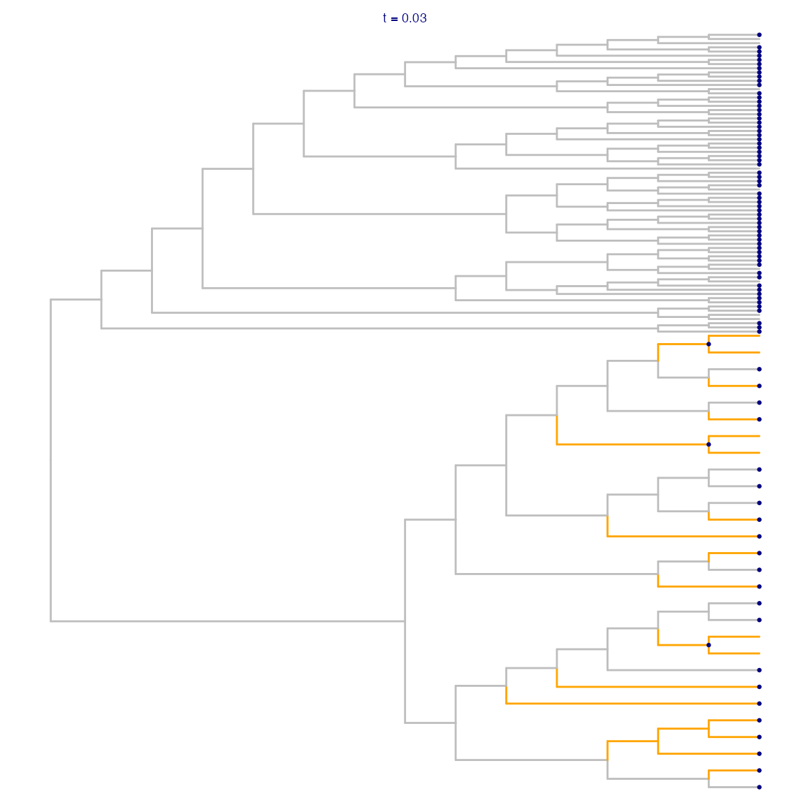
Select the optimal candidate
Finally, given the set of candidates extracted above,treeclimbR can now extract the one providing the optimal aggregation level (Huang et al. 2021).
## Evaluate candidates
da_best <- evalCand(tree = rowTree(da_tse), levels = da_cand$candidate_list,
                    score_data = da_tbl, node_column = "node",
                    p_column = "PValue", sign_column = "logFC")
We can get a summary of all the candidates, as well as an indication of which treeclimbR considers the optimal one, using theinfoCand function:
infoCand(object = da_best)
#>       t    upper_t is_valid method limit_rej level_name  best rej_leaf rej_node
#> 1  0.00 0.02142857     TRUE     BH      0.05          0 FALSE       17       17
#> 2  0.01 0.02142857     TRUE     BH      0.05       0.01  TRUE       17       14
#> 3  0.02 0.02142857     TRUE     BH      0.05       0.02  TRUE       17       14
#> 4  0.03 0.02142857    FALSE     BH      0.05       0.03 FALSE       17       14
#> 5  0.04 0.02142857    FALSE     BH      0.05       0.04 FALSE       17       14
#> 6  0.05 0.04285714    FALSE     BH      0.05       0.05 FALSE       20       14
#> 7  0.10 0.05000000    FALSE     BH      0.05        0.1 FALSE       21       14
#> 8  0.15 0.05000000    FALSE     BH      0.05       0.15 FALSE       21       14
#> 9  0.20 0.05000000    FALSE     BH      0.05        0.2 FALSE       21       14
#> 10 0.25 0.06923077    FALSE     BH      0.05       0.25 FALSE       22       13
#> 11 0.30 0.09166667    FALSE     BH      0.05        0.3 FALSE       23       12
#> 12 0.35 0.10000000    FALSE     BH      0.05       0.35 FALSE       26       13
#> 13 0.40 0.10000000    FALSE     BH      0.05        0.4 FALSE       26       13
#> 14 0.45 0.10000000    FALSE     BH      0.05       0.45 FALSE       26       13
#> 15 0.50 0.10000000    FALSE     BH      0.05        0.5 FALSE       26       13
#> 16 0.55 0.10000000    FALSE     BH      0.05       0.55 FALSE       26       13
#> 17 0.60 0.10000000    FALSE     BH      0.05        0.6 FALSE       26       13
#> 18 0.65 0.10000000    FALSE     BH      0.05       0.65 FALSE       26       13
#> 19 0.70 0.10000000    FALSE     BH      0.05        0.7 FALSE       26       13
#> 20 0.75 0.10000000    FALSE     BH      0.05       0.75 FALSE       26       13
#> 21 0.80 0.10000000    FALSE     BH      0.05        0.8 FALSE       26       13
#> 22 0.85 0.10000000    FALSE     BH      0.05       0.85 FALSE       26       13
#> 23 0.90 0.10000000    FALSE     BH      0.05        0.9 FALSE       26       13
#> 24 0.95 0.10000000    FALSE     BH      0.05       0.95 FALSE       26       13
#> 25 1.00 0.10000000    FALSE     BH      0.05          1 FALSE       22       11
We can also extract a vector of significant nodes from the optimal candidate.
da_out <- topNodes(object = da_best, n = Inf, p_value = 0.05)These nodes can then be indicated in the tree.
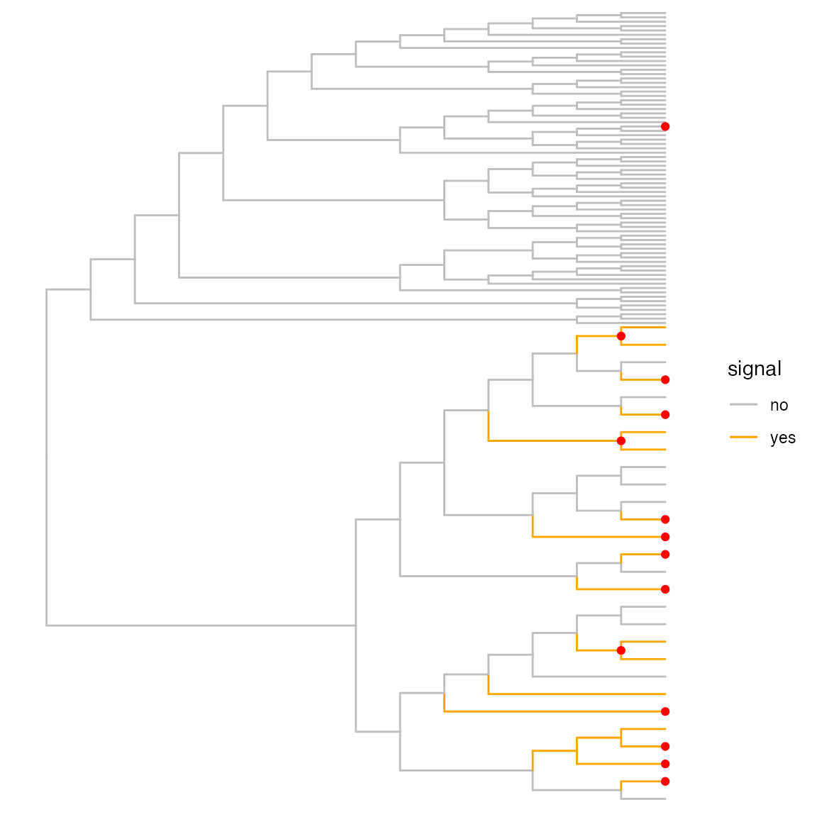
This visualization shows that in most cases, we correctly identify groups of leaves changing synchronously, and we don’t combine true signal nodes with non-changing ones.
In this case, since we are working with simulated data, we can estimate the (leaf-level) false discovery rate and true positive rate for the significant nodes. treeclimbR will automatically extract the descendant leaves for each of the provided nodes, and perform the evaluation on the leaf level.
fdr(rowTree(da_tse), truth = rownames(da_lse)[rowData(da_lse)$Signal],
    found = da_out$node, only.leaf = TRUE)
#>        fdr
#> 0.05882353

tpr(rowTree(da_tse), truth = rownames(da_lse)[rowData(da_lse)$Signal],
    found = da_out$node, only.leaf = TRUE)
#>       tpr
#> 0.8888889
Differential state (DS) analysis
treeclimbR also provides functionality for performing so called ‘differential state analysis’ in a hierarchical setting. An example use case for this type of analysis is in a multi-sample, multi-condition single-cell RNA-seq data set with multiple cell types, where we are interested in finding genes that are differentially expressed between conditions in either a single (high-resolution) cell type (subpopulation) or a group of similar cell subpopulations.
Load and visualize example data
We load a simulated example data set with 20 genes and 500 cells. The cells are assigned to 10 initial (high-resolution) clusters or subpopulations (labelled ‘t1’ to ‘t10’), which are further hierarchically clustered into larger meta-clusters. The hierarchical clustering tree for the subpopulations is provided as the column tree of the TreeSummarizedExperiment object. In addition, the cells come from four different samples (two from condition ‘A’ and two from condition ‘B’). We are interested in finding genes that are differentially expressed between the conditions (so called ‘state markers’) at some level of the clustering tree.
ds_tse <- readRDS(system.file("extdata", "ds_sim_20_500_8de.rds",
                              package = "treeclimbR"))
ds_tse
#> class: TreeSummarizedExperiment
#> dim: 20 500
#> metadata(0):
#> assays(1): counts
#> rownames: NULL
#> rowData names(1): Signal
#> colnames: NULL
#> colData names(3): cluster_id sample_id group
#> reducedDimNames(0):
#> mainExpName: NULL
#> altExpNames(0):
#> rowLinks: NULL
#> rowTree: NULL
#> colLinks: a LinkDataFrame (500 rows)
#> colTree: 1 phylo tree(s) (10 leaves)

## Assignment of cells to high-resolution clusters, samples and conditions
head(colData(ds_tse))
#> DataFrame with 6 rows and 3 columns
#>    cluster_id sample_id       group
#>   <character> <integer> <character>
#> 1          t7         4           B
#> 2          t7         4           B
#> 3          t1         4           B
#> 4          t4         1           A
#> 5          t6         1           A
#> 6          t1         1           A

## Tree providing the successive aggregation of the high-resolution clusters
## into more coarse-grained ones
## Node numbers are indicated in blue, node labels in orange
ggtree(colTree(ds_tse)) +
    geom_text2(aes(label = node), color = "darkblue",
               hjust = -0.5, vjust = 0.7) +
    geom_text2(aes(label = label), color = "darkorange",
               hjust = -0.1, vjust = -0.7)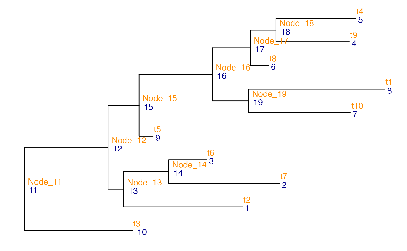
The data set contains 8 genes that are simulated to be differentially expressed between the two conditions. Four genes are differentially expressed in all the clusters, two in clusters t2,t6 and t7, and two in clusters t4and t5.
rowData(ds_tse)[rowData(ds_tse)$Signal != "no", , drop = FALSE]
#> DataFrame with 8 rows and 1 column
#>        Signal
#>   <character>
#> 1         all
#> 2  t2, t6, t7
#> 3         all
#> 4  t2, t6, t7
#> 5         all
#> 6         all
#> 7      t4, t5
#> 8      t4, t5
Aggregate counts for internal nodes
As for the DA analysis, the first step is to aggregate the counts for the internal nodes. In this use case, it effectively corresponds to generating pseudobulk samples for each original sample and each internal node in the tree.
ds_se <- aggDS(TSE = ds_tse, assay = "counts", sample_id = "sample_id",
               group_id = "group", cluster_id = "cluster_id", FUN = sum)
#> Warning in TreeSummarizedExperiment::convertNode(tree = tree, node =
#> as.character(cell_info$cluster_id)): Multiple nodes are found to have the same
#> label.
ds_se
#> class: SummarizedExperiment
#> dim: 20 4
#> metadata(3): experiment_info agg_pars n_cells
#> assays(19): alias_1 alias_2 ... alias_18 alias_19
#> rownames: NULL
#> rowData names(0):
#> colnames(4): 4 1 2 3
#> colData names(1): group
Note how there is now one assay for each node in the tree (ten for the leaves and nine for the internal nodes). Each of these assays contains the aggregated counts for all genes in all cells belonging to the corresponding node, split by sample ID.
This object also stores information about the number of cells contributing to each node and sample
metadata(ds_se)$n_cells
#>            4   1   2   3
#> alias_1   10   8  14  12
#> alias_2   17  12  10  14
#> alias_3    9   9  18  11
#> alias_4   14  13  14   7
#> alias_5   11   9  13  14
#> alias_6   15  14  13  12
#> alias_7   16  18  16  13
#> alias_8   17  13  15   7
#> alias_9    7  12  13  13
#> alias_10  12  11  12  12
#> alias_11 128 119 138 115
#> alias_12 116 108 126 103
#> alias_13  36  29  42  37
#> alias_14  26  21  28  25
#> alias_15  80  79  84  66
#> alias_16  73  67  71  53
#> alias_17  40  36  40  33
#> alias_18  25  22  27  21
#> alias_19  33  31  31  20
Perform differential analysis for leaves and nodes
Next, we perform the differential analysis. As for the DA analysis above, treeclimbR provides a convenience function for applying edgeR on the aggregated counts for each node. However, any suitable method can be used.
ds_res <- runDS(SE = ds_se, tree = colTree(ds_tse), option = "glmQL",
                design = model.matrix(~ group, data = colData(ds_se)),
                contrast = c(0, 1), filter_min_count = 0,
                filter_min_total_count = 1, filter_min_prop = 0, min_cells = 5,
                group_column = "group", message = FALSE)
#> 0 nodes are ignored, as they don't contain at least 5 cells in at least half of the samples.
As before, the output contains the edgeR results for each node, the tree, and the list of nodes that were dropped because of a too low count.
names(ds_res)
#> [1] "edgeR_results" "tree"          "nodes_drop"
names(ds_res$edgeR_results)
#>  [1] "alias_1"  "alias_2"  "alias_3"  "alias_4"  "alias_5"  "alias_6"
#>  [7] "alias_7"  "alias_8"  "alias_9"  "alias_10" "alias_11" "alias_12"
#> [13] "alias_13" "alias_14" "alias_15" "alias_16" "alias_17" "alias_18"
#> [19] "alias_19"
We can create a table with the node results as well. Note that this table contains the results from all genes (features) at all nodes.
ds_tbl <- nodeResult(ds_res, type = "DS", n = Inf)
dim(ds_tbl)
#> [1] 380   7
head(ds_tbl)
#>           logFC   logCPM        F       PValue          FDR node feature
#> 3...1  1.647224 16.31850 2702.109 2.402920e-38 9.131097e-36   11       3
#> 1...2  1.623036 16.28457 2411.255 2.264792e-37 4.303105e-35   11       1
#> 6...3 -1.566550 16.27571 2177.354 1.684458e-36 2.133646e-34   11       6
#> 5...4 -1.528560 16.26806 2042.835 5.892588e-36 5.597959e-34   11       5
#> 6...5 -1.633382 16.19005 1671.077 3.012255e-34 2.289314e-32   13       6
#> 5...6 -1.577632 16.18364 1610.875 6.168542e-34 3.906743e-32   13       5
Find candidates
The next step in the analysis is to generate a list of candidates. This is done separately for each gene - hence, we first split the result table above by the feature column, and then run[getCand()](../reference/getCand.html) for each subtable.
## Split result table by feature
ds_tbl_list <- split(ds_tbl, f = ds_tbl$feature)

## Find candidates for each gene separately
ds_cand_list <- lapply(seq_along(ds_tbl_list),
                       FUN = function(x) {
                           getCand(
                               tree = colTree(ds_tse),
                               t = seq(from = 0.05, to = 1, by = 0.05),
                               score_data = ds_tbl_list[[x]],
                               node_column = "node",
                               p_column = "PValue",
                               sign_column = "logFC",
                               message = FALSE)$candidate_list
                       })
names(ds_cand_list) <- names(ds_tbl_list)
Select the optimal candidate
We can then find the optimal candidate using the[evalCand()](../reference/evalCand.html) function, and list the top hits.
ds_best <- evalCand(tree = colTree(ds_tse), type = "multiple",
                    levels = ds_cand_list, score_data = ds_tbl_list,
                    node_column = "node",
                    p_column = "PValue",
                    sign_column = "logFC",
                    feature_column = "feature",
                    limit_rej = 0.05,
                    message = FALSE,
                    use_pseudo_leaf = FALSE)

ds_out <- topNodes(object = ds_best, n = Inf, p_value = 0.05)
ds_out
#>            logFC   logCPM         F       PValue          FDR node feature
#> 1       1.623036 16.28457 2411.2547 2.264792e-37 4.303105e-35   11       1
#> 2       1.535873 16.20796 1350.8552 1.904533e-32 1.033890e-30   13       2
#> 3       1.647224 16.31850 2702.1091 2.402920e-38 9.131097e-36   11       3
#> 4      -1.613073 16.25077 1258.5324 7.530189e-32 3.576840e-30   13       4
#> 5      -1.528560 16.26806 2042.8352 5.892588e-36 5.597959e-34   11       5
#> 6      -1.566550 16.27571 2177.3536 1.684458e-36 2.133646e-34   11       6
#> 7...7   1.322240 16.11680  501.7687 3.012677e-24 4.770073e-23    5       7
#> 7...8   1.656876 16.10320  630.0092 1.171324e-09 5.634218e-09    9       7
#> 8...9  -1.523605 16.26492  719.5137 3.466238e-27 6.272241e-26    5       8
#> 8...10 -1.685560 16.34385  252.2818 6.672580e-08 2.848967e-07    9       8
#>               adj.p signal.node
#> 1      1.811834e-35        TRUE
#> 2      6.094507e-31        TRUE
#> 3      3.844672e-36        TRUE
#> 4      2.008050e-30        TRUE
#> 5      2.357035e-34        TRUE
#> 6      8.983774e-35        TRUE
#> 7...7  6.025355e-23        TRUE
#> 7...8  2.082354e-08        TRUE
#> 8...9  7.922830e-26        TRUE
#> 8...10 1.067613e-06        TRUE
As expected, we detect the eight truly differentially expressed features (feature 1-8). Furthermore, we see that they have been aggregated to different nodes in the tree. Features 1, 3, 5 and 6 are aggregated to node 11, features 2 and 4 to node 13, and features 7 and 8 to nodes 5 and 9. Let’s see which leaves these internal nodes correspond to.
lapply(findDescendant(colTree(ds_tse), node = c(11, 13, 5, 9),
                      self.include = TRUE,
                      use.alias = FALSE, only.leaf = TRUE),
       function(x) convertNode(colTree(ds_tse), node = x))
#> $Node_11
#>  [1] "t2"  "t7"  "t6"  "t9"  "t4"  "t8"  "t10" "t1"  "t5"  "t3"
#>
#> $Node_13
#> [1] "t2" "t7" "t6"
#>
#> $t4
#> [1] "t4"
#>
#> $t5
#> [1] "t5"
Indeed, comparing this to the ground truth provided above, we see that each gene has been aggregated to the lowest node level that contains all the original subpopulations where the gene was simulated to be differentially expressed between conditions A and B:
rowData(ds_tse)[rowData(ds_tse)$Signal != "no", , drop = FALSE]
#> DataFrame with 8 rows and 1 column
#>        Signal
#>   <character>
#> 1         all
#> 2  t2, t6, t7
#> 3         all
#> 4  t2, t6, t7
#> 5         all
#> 6         all
#> 7      t4, t5
#> 8      t4, t5
Additional examples
Additional examples of applying treeclimbR to experimental data sets can be found on GitHub.
Session info
This document was executed with the following package versions (click to expand)
sessionInfo()
#> R version 4.5.0 Patched (2025-04-15 r88147)
#> Platform: aarch64-apple-darwin20
#> Running under: macOS Sonoma 14.7.4
#>
#> Matrix products: default
#> BLAS:   /Library/Frameworks/R.framework/Versions/4.5-arm64/Resources/lib/libRblas.0.dylib
#> LAPACK: /Library/Frameworks/R.framework/Versions/4.5-arm64/Resources/lib/libRlapack.dylib;  LAPACK version 3.12.1
#>
#> locale:
#> [1] en_US.UTF-8/en_US.UTF-8/en_US.UTF-8/C/en_US.UTF-8/en_US.UTF-8
#>
#> time zone: UTC
#> tzcode source: internal
#>
#> attached base packages:
#> [1] stats4    stats     graphics  grDevices utils     datasets  methods
#> [8] base
#>
#> other attached packages:
#>  [1] ggplot2_3.5.2                   dplyr_1.1.4
#>  [3] ggtree_3.15.0                   treeclimbR_1.5.0
#>  [5] TreeSummarizedExperiment_2.15.1 Biostrings_2.75.4
#>  [7] XVector_0.47.2                  SingleCellExperiment_1.29.2
#>  [9] SummarizedExperiment_1.37.0     Biobase_2.67.0
#> [11] GenomicRanges_1.59.1            GenomeInfoDb_1.43.4
#> [13] IRanges_2.41.3                  S4Vectors_0.45.4
#> [15] BiocGenerics_0.53.6             generics_0.1.3
#> [17] MatrixGenerics_1.19.1           matrixStats_1.5.0
#> [19] BiocStyle_2.35.0
#>
#> loaded via a namespace (and not attached):
#>   [1] RColorBrewer_1.1-3          jsonlite_2.0.0
#>   [3] shape_1.4.6.1               magrittr_2.0.3
#>   [5] TH.data_1.1-3               farver_2.1.2
#>   [7] nloptr_2.2.1                rmarkdown_2.29
#>   [9] GlobalOptions_0.1.2         fs_1.6.6
#>  [11] ragg_1.4.0                  vctrs_0.6.5
#>  [13] minqa_1.2.8                 rstatix_0.7.2
#>  [15] htmltools_0.5.8.1           S4Arrays_1.7.3
#>  [17] broom_1.0.8                 gridGraphics_0.5-1
#>  [19] SparseArray_1.7.7           Formula_1.2-5
#>  [21] sass_0.4.10                 bslib_0.9.0
#>  [23] desc_1.4.3                  plyr_1.8.9
#>  [25] sandwich_3.1-1              zoo_1.8-14
#>  [27] cachem_1.1.0                igraph_2.1.4
#>  [29] lifecycle_1.0.4             iterators_1.0.14
#>  [31] pkgconfig_2.0.3             Matrix_1.7-3
#>  [33] R6_2.6.1                    fastmap_1.2.0
#>  [35] GenomeInfoDbData_1.2.14     rbibutils_2.3
#>  [37] clue_0.3-66                 aplot_0.2.5
#>  [39] digest_0.6.37               colorspace_2.1-1
#>  [41] ggnewscale_0.5.1            patchwork_1.3.0
#>  [43] textshaping_1.0.0           ggpubr_0.6.0
#>  [45] labeling_0.4.3              cytolib_2.19.3
#>  [47] colorRamps_2.3.4            httr_1.4.7
#>  [49] polyclip_1.10-7             abind_1.4-8
#>  [51] compiler_4.5.0              withr_3.0.2
#>  [53] doParallel_1.0.17           ConsensusClusterPlus_1.71.0
#>  [55] backports_1.5.0             BiocParallel_1.41.5
#>  [57] viridis_0.6.5               carData_3.0-5
#>  [59] ggforce_0.4.2               ggsignif_0.6.4
#>  [61] MASS_7.3-65                 DelayedArray_0.33.6
#>  [63] rjson_0.2.23                FlowSOM_2.15.0
#>  [65] diffcyt_1.27.3              tools_4.5.0
#>  [67] ape_5.8-1                   glue_1.8.0
#>  [69] nlme_3.1-168                grid_4.5.0
#>  [71] Rtsne_0.17                  reshape2_1.4.4
#>  [73] cluster_2.1.8.1             gtable_0.3.6
#>  [75] tidyr_1.3.1                 car_3.1-3
#>  [77] stringr_1.5.1               foreach_1.5.2
#>  [79] pillar_1.10.2               yulab.utils_0.2.0
#>  [81] limma_3.63.13               circlize_0.4.16
#>  [83] splines_4.5.0               flowCore_2.19.0
#>  [85] tweenr_2.0.3                treeio_1.31.0
#>  [87] lattice_0.22-7              survival_3.8-3
#>  [89] dirmult_0.1.3-5             RProtoBufLib_2.19.0
#>  [91] tidyselect_1.2.1            ComplexHeatmap_2.23.1
#>  [93] locfit_1.5-9.12             knitr_1.50
#>  [95] gridExtra_2.3               reformulas_0.4.0
#>  [97] bookdown_0.43               edgeR_4.5.10
#>  [99] xfun_0.52                   statmod_1.5.0
#> [101] stringi_1.8.7               UCSC.utils_1.3.1
#> [103] ggfun_0.1.8                 lazyeval_0.2.2
#> [105] yaml_2.3.10                 boot_1.3-31
#> [107] evaluate_1.0.3              codetools_0.2-20
#> [109] tibble_3.2.1                BiocManager_1.30.25
#> [111] ggplotify_0.1.2             cli_3.6.4
#> [113] systemfonts_1.2.2           Rdpack_2.6.4
#> [115] munsell_0.5.1               jquerylib_0.1.4
#> [117] Rcpp_1.0.14                 png_0.1-8
#> [119] XML_3.99-0.18               parallel_4.5.0
#> [121] pkgdown_2.1.1.9000          lme4_1.1-37
#> [123] viridisLite_0.4.2           mvtnorm_1.3-3
#> [125] tidytree_0.4.6              scales_1.3.0
#> [127] purrr_1.0.4                 crayon_1.5.3
#> [129] GetoptLong_1.0.5            rlang_1.1.6
#> [131] multcomp_1.4-28
References
Huang, Ruizhu, Charlotte Soneson, Pierre-Luc Germain, Thomas S B Schmidt, Christian Von Mering, and Mark D Robinson. 2021.“treeclimbR Pinpoints the Data-Dependent Resolution of Hierarchical Hypotheses.” Genome Biology 22 (1): 157.