Jupyter Notebook | kepler.gl (original) (raw)
Jupyter Notebook
Last updated 6 months ago
kepler.gl for Jupyter User Guide
To install use pip:
If you're on Mac, used pip install, and you're running Notebook 5.3 and above, you don't need to run the following:
$ jupyter nbextension install --py --sys-prefix keplergl # can be skipped for notebook 5.3 and above
$ jupyter nbextension enable --py --sys-prefix keplergl # can be skipped for notebook 5.3 and above
Then install jupyter labextension.
$ jupyter labextension install @jupyter-widgets/jupyterlab-manager keplergl-jupyterPrerequisites for JupyterLab
- Input:
**height**optional default:400
Height of the map display**use_arrow**booloptional default:False
Allow load and render data faster using GeoArrow**config**dictoptional
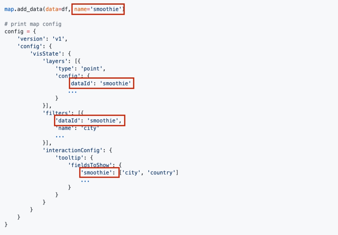
Map config as a dictionary. ThedataIdin the layer and filter settings should match thenameof the dataset they are created under
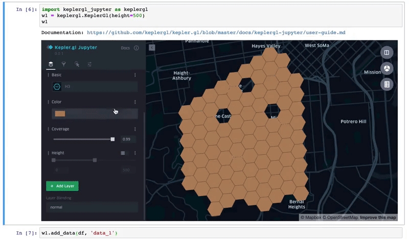
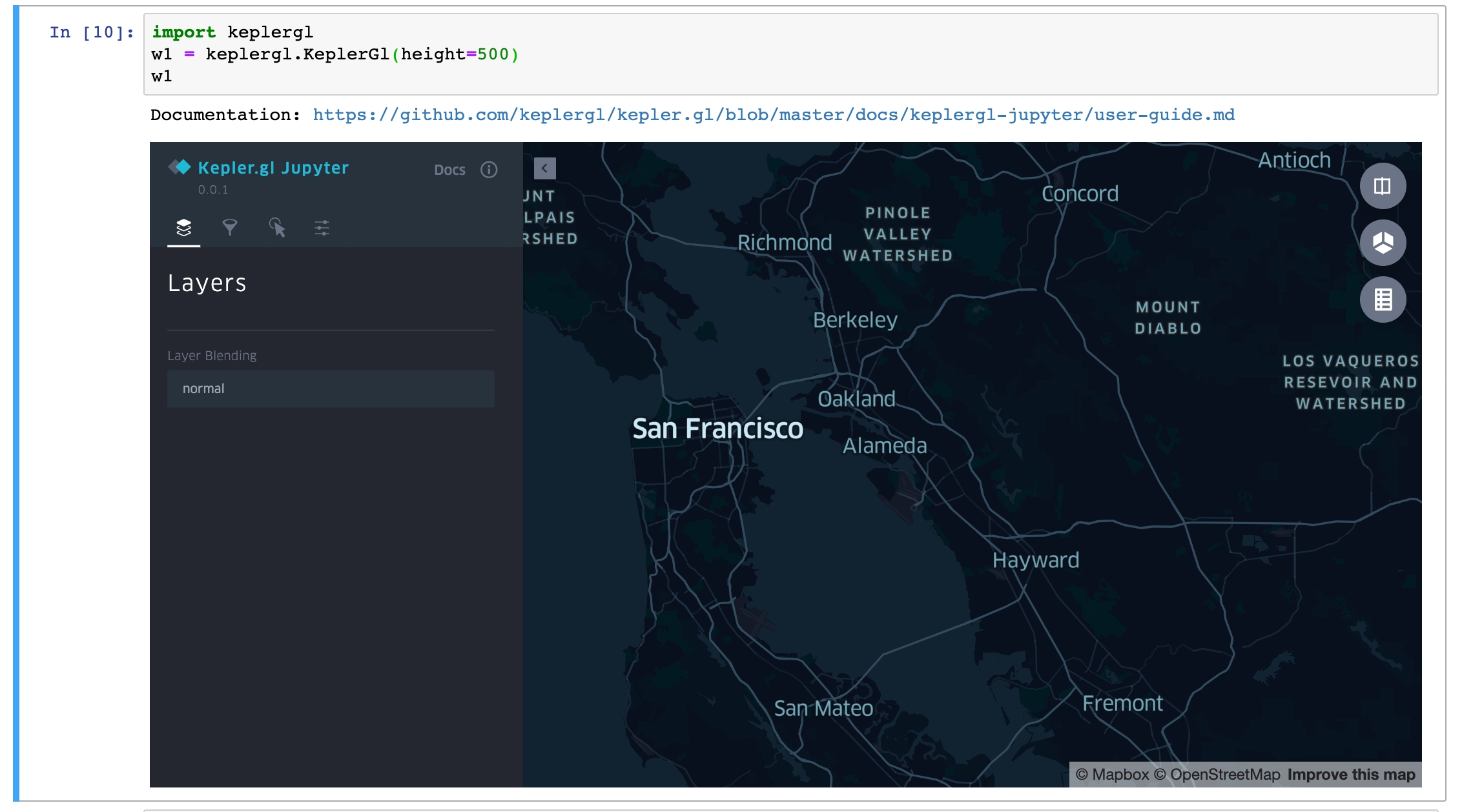
The following command will load kepler.gl widget below a cell. The map object created here is **map_1** it will be used throughout the code example in this doc.
# Load an empty map
from keplergl import KeplerGl
map_1 = KeplerGl()
map_1
# Load a map with data and config and height
from keplergl import KeplerGl
map_2 = KeplerGl(height=400, data={"data_1": my_df}, config=config)
map_2- Inputs
**name**required Name of the data entry.**use_arrow**optional Allow load and render data faster using GeoArrow.
name of the dataset will be the saved to the dataId property of each layer, filter and interactionConfig in the config.
kepler.gl expected the data to be CSV, GeoJSON, DataFrame or GeoDataFrame. You can call **add_data** multiple times to add multiple datasets to kepler.gl
# DataFrame
df = pd.read_csv('hex-data.csv')
map_1.add_data(data=df, name='data_1')
# CSV
with open('csv-data.csv', 'r') as f:
csvData = f.read()
map_1.add_data(data=csvData, name='data_2')
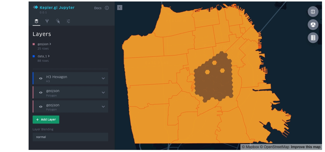
# GeoJSON as string
with open('sf_zip_geo.json', 'r') as f:
geojson = f.read()
map_1.add_data(data=geojson, name='geojson')Print the current data added to the map. As a Dict
map_1.data
# {'data_1': 'hex_id,value\n89283082c2fffff,64\n8928308288fffff,73\n89283082c07ffff,65\n89283082817ffff,74\n89283082c3bffff,66\n8...`,
#  'data_3': 'location, lat, lng, name\n..',
#  'data_3': '{"type": "FeatureCollecti...'}
kepler.gl supports CSV, GeoJSON, Pandas DataFrame or GeoPandas GeoDataFrame.
You can create a CSV string by reading from a CSV file.
with open('csv-data.csv', 'r') as f:
    csvData = f.read()
# csvData = "hex_id,value\n89283082c2fffff,64\n8928308288fffff,73\n89283082c07ffff,65\n89283082817ffff,74\n89283082c3bffff,66\n8..."
map_1.add_data(data=csvData, name='data_2')
feature = {
"type": "Feature",
"properties": {"name": "Coors Field"},
"geometry": {"type": "Point", "coordinates": [-104.99404, 39.75621]}
}
featureCollection = {
"type": "FeatureCollection",
"features": [{
"type": "Feature",
"geometry": {"type": "Point", "coordinates": [102.0, 0.5]},
"properties": {"prop0": "value0"}
}]
}
map_1.add_data(data=feature, name="feature")
map_1.add_data(data=featureCollection, name="feature_collection")# GeoJson Feature geometry
geometryString = {
'type': 'Polygon',
'coordinates': [[[-74.158491,40.835947],[-74.148473,40.834522],[-74.142598,40.833128],[-74.151923,40.832074],[-74.158491,40.835947]]]
}
# create json string
json_str = json.dumps(geometryString)
# create data frame
df_with_geometry = pd.DataFrame({
'id': [1],
'geometry_string': [json_str]
})
# add to map
map_1.add_data(df_with_geometry, "df_with_geometry")df = pd.DataFrame(
{'City': ['Buenos Aires', 'Brasilia', 'Santiago', 'Bogota', 'Caracas'],
'Latitude': [-34.58, -15.78, -33.45, 4.60, 10.48],
'Longitude': [-58.66, -47.91, -70.66, -74.08, -66.86]})
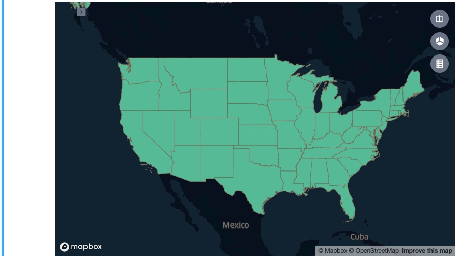
w1.add_data(data=df, name='cities')url = 'http://eric.clst.org/assets/wiki/uploads/Stuff/gz_2010_us_040_00_500k.json'
country_gdf = geopandas.read_file(url)
w1.add_data(data=country_gdf, name="state")# WKT
wkt_str = 'POLYGON ((-74.158491 40.835947, -74.130031 40.819962, -74.148818 40.830916, -74.151923 40.832074, -74.158491 40.835947))'
df_w_wkt = pd.DataFrame({
'id': [1],
'wkt_string': [wkt_str]
})
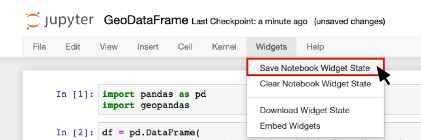
map_1.add_data(df_w_wkt, "df_w_wkt")Interact with kepler.gl and customize layers and filters. Map data and config will be stored locally to the widget state. To make sure the map state is saved, select Widgets > Save Notebook Widget State, before shutting down the kernel.
you can print your current map configuration at any time in the notebook
map_1.config
## {u'config': {u'mapState': {u'bearing': 2.6192893401015205,
#  u'dragRotate': True,
#   u'isSplit': False,
#   u'latitude': 37.76209132041332,
#   u'longitude': -122.42590232651203,
Apply config to a map:
- Directly apply config to the map.
config = {
    'version': 'v1',
    'config': {
        'mapState': {
            'latitude': 37.76209132041332,
            'longitude': -122.42590232651203,
            'zoom': 12.32053899007826
        }
        ...
    }
},
map_1.add_data(data=df, name='data_1')
map_1.config = config- Load it when creating the map
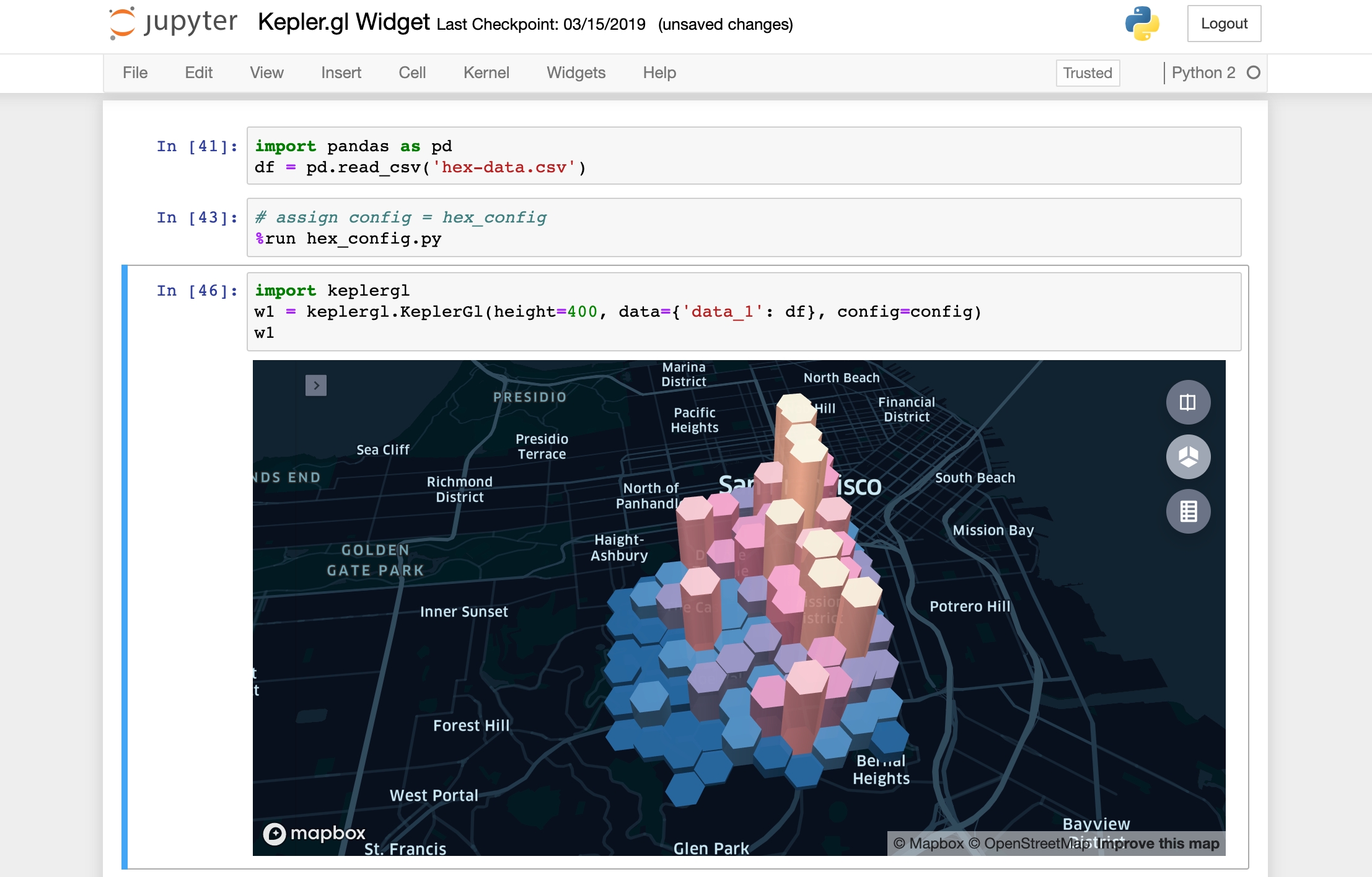
map_1 = KeplerGl(height=400, data={'data_1': my_df}, config=config)If want to load the map next time with this saved config, the easiest way to do is to save the it to a file and use the magic command %run to load it w/o cluttering up your notebook.
# Save map_1 config to a file
with open('hex_config.py', 'w') as f:
   f.write('config = {}'.format(map_1.config))

# load the config
%run hex_config.py
6. Match config with data
All layers, filters and tooltips are associated with a specific dataset. Therefore the data and config in the map has to be able to match each other. The name of the dataset is assigned to:
- key in
interactionConfig.tooltip.fieldToShow.
You can use the same config on another dataset with the same name and schema.
When you click in the map and change settings, config is saved to widget state. Closing the notebook and reopen it will reload current map. However, you need to manually select Widget > Save Notebook Widget State before shut downing the kernel to make sure it will be reloaded.
- input
**data**: optional A data dictionary {"name": data}, if not provided, will use current map data**config**: optional map config dictionary, if not provided, will use current map config**file_name**: optional the html file name, default iskeplergl_map.html**read_only**: optional ifread_onlyisTrue, hide side panel to disable map customization
You can export your current map as an interactive html file.
# this will save current map
map_1.save_to_html(file_name='first_map.html')

# this will save map with provided data and config
map_1.save_to_html(data={'data_1': df}, config=config, file_name='first_map.html')

# this will save map with the interaction panel disabled
map_1.save_to_html(file_name='first_map.html', read_only=True)- input
**data**: optional A data dictionary {"name": data}, if not provided, will use current map data**config**: optional map config dictionary, if not provided, will use current map config**read_only**: optional ifread_onlyisTrue, hide side panel to disable map customization
You can also directly serve the current map via a flask app. To do that return kepler’s map HTML representation. Here is an example on how to do that:
from flask import Flask

app = Flask(__name__)

@app.route('/')
def index():
    return map_1._repr_html_()

if __name__ == '__main__':
    app.run(debug=True)
1. What about Microsoft Windows?
2. Install keplergl-jupyter on Jupyter Lab failed?
Run jupyter labextension install keplergl-jupyter --debug and copy console output before creating an issue.
If you are running install and uninstall several times. You should run.
jupyter lab clean
jupyter lab build
2.1 JavaScript heap out of memory when installing lab extension
If you see this error during install labextension
$ FATAL ERROR: CALL_AND_RETRY_LAST Allocation failed - JavaScript heap out of memoryrun
$ export NODE_OPTIONS=--max-old-space-size=40963. Is my lab extension successfully installed?
Run jupyter labextension list You should see below. (Version may vary)
JupyterLab v1.1.4
Known labextensions:
   app dir: /Users/xxx/jupyter-python3/ENV3/share/jupyter/lab
        @jupyter-widgets/jupyterlab-manager v1.0.2  enabled  OK
        keplergl-jupyter v0.1.0  enabled  OK
4. What's your python and node env
Python
python==3.7.4
notebook==6.0.3
jupyterlab==2.1.2
ipywidgets==7.5.1
Node (Only for JupyterLab)
If you are using Jupyter Lab, you will also need to install the JupyterLab extension. This require > 10.15.0
Datasets as a dictionary, key is the name of the dataset. Read more on
By default, the User Guide URL () will be printed when a map is created. To hide the User Guide URL, set show_docs=False.
You can also create the map and pass in the data or data and config at the same time. Follow the instruction to
Load map with data and config
**data** required CSV, GeoJSON or DataFrame. Read more on
According to : GeoJSON is a format for encoding a variety of geographic data structures. A GeoJSON object may represent a region of space (a Geometry), a spatially bounded entity (a Feature), or a list of Features (a FeatureCollection). GeoJSON supports the following geometry types: Point, LineString, Polygon, MultiPoint, MultiLineString, MultiPolygon, and GeometryCollection. Features in GeoJSON contain a Geometry object and additional properties, and a FeatureCollection contains a list of Features.
kepler.gl supports all the GeoJSON types above excepts GeometryCollection. You can pass in either a single or a . You can format the GeoJSON either as a string or a dict type
Geometries (Polygons, LindStrings) can be embedded into CSV or DataFrame with a Json string. Use the geometry property of a , which includes type and coordinates.
kepler.gl accepts , it automatically converts the current geometry column from shapely to wkt string and re-projects geometries to latitude and longitude (EPSG:4326) if the active geometry column is in a different projection.
You can embed geometries (Polygon, LineStrings etc) into CSV or DataFrame using
When the map is final, you can copy this config and load it later to reproduce the same map. Follow the instruction to .
: Load kepler.gl widget, add data and config
: Embed Polygon geometries as GeoJson and WKT inside a CSV
: Load GeoJSON to kepler.gl
: Load DataFrame to kepler.gl
: Load GeoDataFrame to kepler.gl
keplergl is currently only published to PyPI, and unfortunately I use a Mac. If you encounter errors installing it on windows, might shed some light. Follow this issue for support.
Make sure you are using node 8.15.0. and you have installed @jupyter-widgets/jupyterlab-manager. Depends on your JupyterLab version. You might need to install the specific version of . with jupyter labextension install @jupyter-widgets/jupyterlab-manager@0.31. When use it in Jupyter lab, keplergl is only supported in JupyterLab > 1.0 and Python 3.