scipy.stats.logistic — SciPy v1.16.2 Manual (original) (raw)

scipy.stats.logistic = <scipy.stats._continuous_distns.logistic_gen object>[source]#

A logistic (or Sech-squared) continuous random variable.

As an instance of the rv_continuous class, logistic object inherits from it a collection of generic methods (see below for the full list), and completes them with details specific for this particular distribution.

Methods

Notes

The probability density function for logistic is:

\[f(x) = \frac{\exp(-x)} {(1+\exp(-x))^2}\]

logistic is a special case of genlogistic with c=1.

Remark that the survival function (logistic.sf) is equal to the Fermi-Dirac distribution describing fermionic statistics.

The probability density above is defined in the “standardized” form. To shift and/or scale the distribution use the loc and scale parameters. Specifically, logistic.pdf(x, loc, scale) is identically equivalent to logistic.pdf(y) / scale withy = (x - loc) / scale. Note that shifting the location of a distribution does not make it a “noncentral” distribution; noncentral generalizations of some distributions are available in separate classes.

Examples

import numpy as np from scipy.stats import logistic import matplotlib.pyplot as plt fig, ax = plt.subplots(1, 1)

Get the support:

lb, ub = logistic.support()

Calculate the first four moments:

mean, var, skew, kurt = logistic.stats(moments='mvsk')

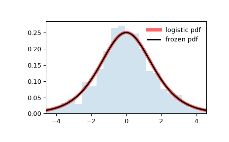
Display the probability density function (pdf):

x = np.linspace(logistic.ppf(0.01), ... logistic.ppf(0.99), 100) ax.plot(x, logistic.pdf(x), ... 'r-', lw=5, alpha=0.6, label='logistic pdf')

Alternatively, the distribution object can be called (as a function) to fix the shape, location and scale parameters. This returns a “frozen” RV object holding the given parameters fixed.

Freeze the distribution and display the frozen pdf:

rv = logistic() ax.plot(x, rv.pdf(x), 'k-', lw=2, label='frozen pdf')

Check accuracy of cdf and ppf:

vals = logistic.ppf([0.001, 0.5, 0.999]) np.allclose([0.001, 0.5, 0.999], logistic.cdf(vals)) True

Generate random numbers:

r = logistic.rvs(size=1000)

And compare the histogram:

ax.hist(r, density=True, bins='auto', histtype='stepfilled', alpha=0.2) ax.set_xlim([x[0], x[-1]]) ax.legend(loc='best', frameon=False) plt.show()