Sensitivity of global warming to the pattern of tropical ocean warming (original) (raw)
Abstract
The current generations of climate models are in substantial disagreement as to the projected patterns of sea surface temperatures (SSTs) in the Tropics over the next several decades. We show that the spatial patterns of tropical ocean temperature trends have a strong influence on global mean temperature and precipitation and on global mean radiative forcing. We identify the SST patterns with the greatest influence on the global mean climate and find very different, and often opposing, sensitivities to SST changes in the tropical Indian and West Pacific Oceans. Our work stresses the need to reduce climate model biases in these sensitive regions, as they not only affect the regional climates of the nearby densely populated continents, but also have a disproportionately large effect on the global climate.
Access this article
Subscribe and save
- Get 10 units per month
- Download Article/Chapter or eBook
- 1 Unit = 1 Article or 1 Chapter
- Cancel anytime Subscribe now
Buy Now
Price excludes VAT (USA)
Tax calculation will be finalised during checkout.
Instant access to the full article PDF.
Notes
- The specific model version was ccm3.10.11.brnchT.366physics.7.
- The normalized optimal SST pattern (denoted “pattern I” in Table 1) is given by\(T_{\rm opt}=S\left(\frac{1}{A_P}\int\limits_P {S^2\;\hbox{d}A}\right)^{-1/2},\) where A P is the area spanned by the patches.
- The sensitivities shown in Fig. 5 are the result of the global response to a local SST change. For comparison, the baseline temperature sensitivity, obtained by taking the global average of only the local prescribed sea surface warming or cooling for a single patch, is 1/A e (about 2 × 10⁻⁹ km−2 in the units of Fig. 5a) where A e is the surface area of the Earth.
References
- Alexander MA, Blade I, Newman M, Lanzante JR, Lau NC, Scott JD (2002) The atmospheric bridge: the influence of ENSO teleconnections on air–sea interaction over the global oceans. J Clim 15:2205–2231
Article Google Scholar - Barsugli JJ, Sardeshmukh PD (2002) Global atmospheric sensitivity to tropical SST anomalies throughout the Indo-Pacific basin. J Clim 15:3427–3442
Article Google Scholar - Bony S, Lau KM, Sud YC (1997) Sea surface temperature and large-scale circulation influences on tropical greenhouse effect and cloud radiative forcing. J Clim 10:2055–2077
Article Google Scholar - Branstator G (1985) Analysis of general circulation model sea-surface temperature anomaly simulations using a linear model. Part I: forced solutions. J Atmos Sci 42:2225–2241
Article Google Scholar - Cess RD, Zhang MH, Ingram WJ, Potter GL, Alekseev V, Barker HW, Cohen-Solal E, Colman RA, Dazlich DA, Del Genio AD, Dix MR, Esch M, Fowler LD, Fraser JR, Galin V, Gates WL, Hack JJ, Kiehl JT, Le Treut H, Lo KKW, McAvaney BJ, Meleshko VP, Morcrette JJ, Randall DA, Roeckner E, Royer JF, Schlesinger ME, Sporyshev PV, Timbal B, Volodin EM, Taylor KE, Wang W, Wetherald RT (1996) Cloud feedback in atmospheric general circulation models: an update. J Geophys Res 101:12791–12794
Article Google Scholar - Colman RA, McAvaney BJ (1997) A study of general circulation model climate feedbacks determined from perturbed sea surface temperature experiments. J Geophys Res 102:19383–19402
Article Google Scholar - Compo GP, Sardeshmukh PD (2004) Storm track predictability on seasonal and decadal scales. J Clim 17:3701–3720
Article Google Scholar - Covey C, AchutaRao KM, Cubasch U, Jones P, Lambert SJ, Mann ME, Phillips TJ, Taylor KE (2003) An overview of results from the coupled model intercomparison project. Global Planet Change 37:103–133
Article Google Scholar - Cubasch U, Meehl GA (2001) Projections of future climate change. In: Houghton JT et al. (eds) Climate change 2001: the scientific basis. Cambridge University Press, Cambridge, UK, pp 526–582
Google Scholar - Goddard L, Mason SJ, Zebiak SE, Ropelewski CF, Basher R, Cane MA (2001) Current approaches to seasonal-to-interannual climate predictions. Int J Climatol 21:1111–1152
Article Google Scholar - Gu C (1989) RKPACK and its applications: fitting smoothing spline models. Proc. Stat. Comp. Sec., American Statistical Society, 42–51
- Hartmann DL, Michelsen ML (1993) Large-scale effects on the regulation of tropical sea surface temperature. J Clim 6:2049–2062
Article Google Scholar - Hurrell JW, Hoerling MP, Phillips AS, Xu T (2005) Twentieth century North Atlantic climate change. Part I: assessing determinism. Clim Dynam 23:371–389
Google Scholar - Inamdar AK, Ramanathan V (1998) Tropical and global scale interactions among water vapor, atmospheric greenhouse effect, and surface temperature. J Geophys Res 103:32177–32194
Article Google Scholar - Kinter J, Folland CK, Kirtman BP (2005) Final report of the workshop on climate of the 20th century and seasonal to interannual climate prediction. Prague, Czech Republic, 4–6 July 2005 (Available at ftp://www.iges.org/pub/kinter/c20c/jul2005/C20C_Wkshp_Jul05_rep.pdf)
- Lau NC, Nath MJ (1994) A modeling study of the relative roles of tropical and extratropical SST anomalies in the variability of the global atmosphere-ocean system. J Clim 7:1184–1207
Article Google Scholar - Newman M, Sardeshmukh PD (1998) The impact of the annual cycle on the North Pacific/North American response to remote low frequency forcing. J Atmos Sci 55:1336–1353
Article Google Scholar - Penland C, Sardeshmukh PD (1995) The optimal growth of tropical sea surface temperature anomalies. J Clim 8:1999–2024
Article Google Scholar - Ramanathan V, Collins W (1991) Thermodynamic regulation of ocean warming by cirrus clouds deduced from observations of the 1987 El Niño. Nature 351:27–32
Article Google Scholar - Rayner NA, Parker DE, Horton EB, Folland CK, Alexander LV, Rowell DP, Kent EC, Kaplan A (2003) Global analyses of sea surface temperature, sea ice, and night marine air temperature since the late nineteenth century. J Geophys Res 108:4407–4443 (doi:10.1029/2002JD002670)
Google Scholar - Saravanan R (1998) Atmospheric low-frequency variability and its relationship to mid latitude SST variability: studies using the NCAR climate system model. J Clim 11:1386–1404
Article Google Scholar - Sardeshmukh PD, Hoskins BJ (1988) The generation of global rotational flow by steady idealized tropical divergence. J Atmos Sci 45:1228–1251
Article Google Scholar - Schneider EK, Lindzen RS, Kirtman BP (1997) A tropical influence on global climate. J Atmos Sci 54:1349–1358
Article Google Scholar - Soden BJ (1997) Variations in the tropical greenhouse effect during El Niño. J Clim 10:1050–1055
Article Google Scholar - Sun DZ, Fasullo J, Zhang T, Roubicek A (2003) On the radiative and dynamical feedbacks over the equatorial pacific cold tongue. J Clim 16:2425–2432
Article Google Scholar - Ting M, Sardeshmukh PD (1993) Factors determining the extratropical response to equatorial diabatic heating anomalies. J Atmos Sci 50:907–918
Article Google Scholar - Yao MS, Del Genio AD (2002) Effects of cloud parameterization on the simulation of climate changes in the GISS GCM. Part II: sea surface temperature and cloud feedbacks. J Clim 15:2491–2503
Article Google Scholar
Acknowledgments
This work was supported in part by a grant from NOAA’s Office of Global Programs, but does not reflect the official position of NOAA or of the US Government. We thank Jeffrey Yin for help with accessing the IPCC model output and Gil Compo for his assistance. We also appreciate the insightful comments of the two anonymous reviewers.
Author information
Authors and Affiliations
- CIRES Climate Diagnostics Center and NOAA Earth System Research Laboratory, 325 Broadway, R/PSD1, Boulder, CO, 80305-3328, USA
Joseph J. Barsugli, Sang-Ik Shin & Prashant D. Sardeshmukh
Authors
- Joseph J. Barsugli
You can also search for this author inPubMed Google Scholar - Sang-Ik Shin
You can also search for this author inPubMed Google Scholar - Prashant D. Sardeshmukh
You can also search for this author inPubMed Google Scholar
Corresponding author
Correspondence toJoseph J. Barsugli.
Appendix A: smoothing of the sensitivity maps
Appendix A: smoothing of the sensitivity maps
A thin-plate spatial smoothing spline based on the signal-to-noise ratio (Gu 1989) was applied to the climate sensitivites to ensure that only statistically robust features were retained in the sensitivity map. The smoothing parameter used in the spline calculation was based on an a-priori estimate of the expected variance of the ensemble mean responses. This procedure fits a smooth surface to the sampled data so that the variance of the residuals is consistent with the expected variance at the sampling locations. In this manner, variations among nearby data points that could have arisen merely by chance are smoothed out, and the effective sample size at these points is increased. For global sensitivity, the expected variance was taken to be the variance from the 100-year climatological SST control run divided by the sample size (the ensemble size times the number of seasons). Because the variance of precipitation over a patch will likely depend strongly on the total precipitation signal for that patch, the expected variance for the local sensitivities were calculated separately for each patch from the intraensemble variance. In practice the smoothing results in only small changes to the sensitivity maps shown in this paper. For example, Fig. 9 shows the actual values of the sensitivities used in constructing Fig. 4 before smoothing and contouring.
Fig. 9
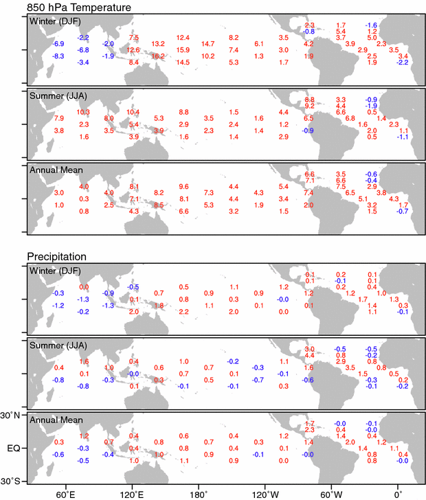
Unsmoothed values of the sensitivity of lower tropospheric temperature (850 hPa pressure level) and precipitation corresponding to the smoothed values contoured in Fig. 4. The numerical values of the sensitivity are shown in text at the center of each patch (red = positive, blue = negative). Units are as in Fig. 4
Rights and permissions
About this article
Cite this article
Barsugli, J.J., Shin, SI. & Sardeshmukh, P.D. Sensitivity of global warming to the pattern of tropical ocean warming.Clim Dyn 27, 483–492 (2006). https://doi.org/10.1007/s00382-006-0143-7
- Received: 27 September 2005
- Accepted: 20 March 2006
- Published: 22 April 2006
- Issue Date: October 2006
- DOI: https://doi.org/10.1007/s00382-006-0143-7