Automata-based monitoring for LTL-FO ^+$$ (original) (raw)

Appendix

We include in this appendix complete version of proofs and theorems that have been elided from the paper out of space considerations as a courtesy for the reviewers. While the paper itself is self-contained and complete, the materiel in this appendix may provide precisions.

We begin in Sect. A.1 with some preliminary notions related to multiset theory, which will be of use in the proof. The main theorem of this paper is also stated in this initial section. Section A.2 provides a supporting lemma related to multiset manipulation. Section A.3 provides the proof of correction of the verification algorithm stated in Sect. 4. Section A.4 includes pseudocode for an auxiliary algorithm referred to in Sect. 4, which was elided from the main paper out of space considerations.

1.1 Preliminaries

In what follows, we represent a slice, which is a nonempty collection of pairs, as a multiset of pairs. Analogously, we represent a SliceSet, which is a nonempty collection of slices, as a multiset of slices. A multiset is a generalized set that allows multiple occurrences of any element (see [26] for reference). Multisets naturally support duplicate run trees (i.e., repeated slices in a SliceSet) and duplicate branches (i.e., repeated pairs in a slice). Thus, they accurately describe the execution of the alternating automata. Although it is obvious that duplicates can be ignored for memory optimization (as was the case in [[11](/article/10.1007/s10009-020-00566-z#ref-CR11 "Finkbeiner, B., Sipma, H.: Checking finite traces using alternating automata. Formal Methods Syst. Des. 24(2), 101–127 (2004). https://doi.org/10.1023/B:FORM.0000017718.28096.48

            ")\] where sets are favored over multisets or the software Pelota presented in Sect. [5](/article/10.1007/s10009-020-00566-z#Sec8)), it is easier, for our correctness proof to keep them.

We mathematically define $\vee $ and $\wedge $ over SliceSets w.r.t. operator $\uplus $ that denotes the sum of two multisets. For any multisets A and B, the sum $A \uplus B$ is a multiset that contains every occurrence of every element of A and B. In other words, the number of occurrences of any element in $A \uplus B$ is equal to the sum of number of occurrences of this element in A and in B. This definition of $\vee $ and $\wedge $ is consistent with our intuitive understanding of SliceSet manipulations: For instance, SliceSet $A \vee B$ equals $\top $ iff A or B does and that it equals $\bot $ iff A and B do. Likewise, the semantics of $\wedge $ ensure that a SliceSet $A \wedge B$ induces $\top $ iff A and B do, and it induces $\bot $ iff A or B does.

Definition 11

Let $A = \{A_1, \ldots , A_m\}$ and $B = \{B_1, \ldots , B_n\}$ be SliceSets:

$A \vee B = A \uplus B=\{A_1, \ldots , A_m, B_1, \ldots , B_n \}$;
$A \wedge B = \{A_i \uplus B_j \mid 1 \le i \le m, 1 \le j \le n\}$.

Next, we introduce the function , a straight copy of 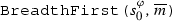with the only difference that is initially assigned to $\{\{ (p, s_0^{\varphi }) \}\}$ instead of $\{\{ ([], s_0^{\varphi }) \}\}$, where $p :V \rightarrow D$ is a partial function that assigns the free variables in $\varphi $ and $s_0^{\varphi }$ is the initial state, representing the entire property ($\varphi $). This notation will allow us to reason about the behavior of the algorithm during intermediate phases in which it manipulates subformulae of $\varphi $ containing free variables. We say that $(p, \varphi )$ is a well-formed formula iff every free variable occurring in $\varphi $ is assigned a value in p. Following the semantics in Sect. 2, for any nonempty finite trace $\overline{m}$ and any well-formed formula $(p, \varphi )$, $[\overline{m} \models (p, \varphi )]$ is equal to $[\overline{m} \models \varphi (p)]$.

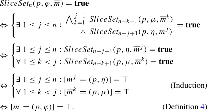
In this context, we can now restate the theorem establishing the correctness of the algorithm presented in Sect. 4 in the slightly modified form that follows when $p = []$ and $\varphi $ is devoid of free variables:

Theorem 2

Let $\overline{m} = m_1, \ldots , m_n$ be a finite message trace, and let $(p, \varphi )$ be a well-formed formula. The output of is equal to $\top $ (resp.$\bot $) iff $[\overline{m} \models (p, \varphi )]= \top $ (resp. $[\overline{m} \models (p, \varphi )]= \bot $).

Observe that if $[\overline{m} \models (p, \varphi )]$ evaluates to ‘?,’ the breath-first algorithm returns a mustiest of multisets of values, in which it requires for the evaluation of the formula to proceed to the next message of the sequence. However, if the final message of the input sequence has been reached, any value returned by different from $\top $ or $\bot $ can be trivially converted to ‘?,’ allowing the verdict of the verification algorithm to correspond to the semantics of LTL-FO$^+$ in all cases. The remainder of this section is devoted to the proof of Theorem 2. We proceed by strong induction on the size of formulae. Recall that the size of a formula $\varphi $, denoted by $|\varphi |$, is the height of its tree decomposition. The recursive nature of the algorithms favors this decision: The size of the input of is reduced by 1 size unit with each recursive call.

1.2 Lemma on SliceSets

In what follows, we omit the subscripted index of the slice and SliceSet when it is clear from context. The following notation identifies specific s (or terms) computed by :

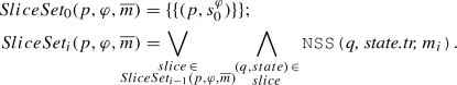
Definition 12

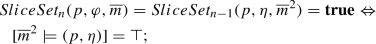
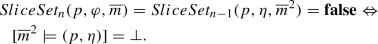
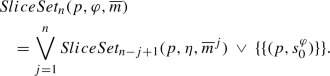
Let $(p, \varphi )$ be a well-formed formula, and let $\overline{m} = m_1, \ldots , m_n$ ($n \ge 0$) be a finite message trace. The sequence of SliceSets and truth values ($\mathbf {true}$, $\mathbf {false}$) is recursively defined as follows:

The following lemma describes more formally the relationship between s and the algorithm.

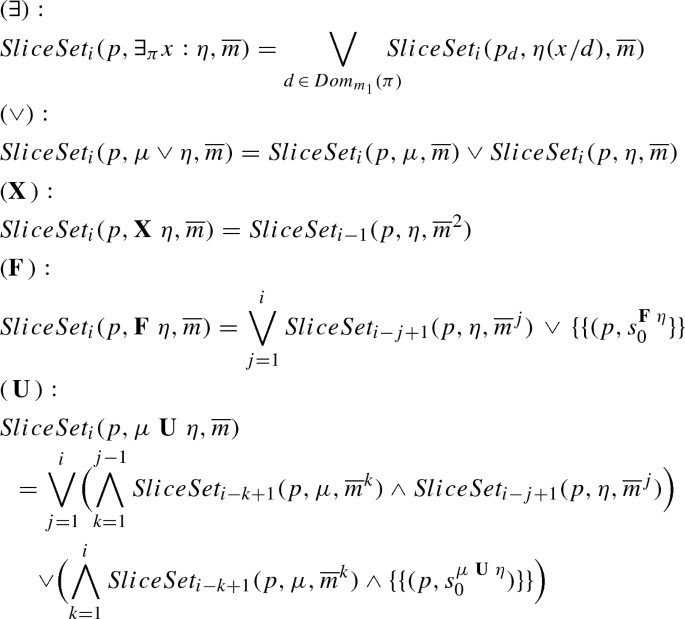
Lemma 1

Let $\mu $ and $\eta $ be formulae. Let $p :{V \setminus \{x\}} \rightarrow D$ be a partial function, and for all $d \in D$, denote $p \cup \{(x, d)\}$ by the shorthand $p_{d}$. If the expressions $(p_{d}, \eta )$, $(p, \eta )$ and $(p, \mu )$ are well formed, then for any path $\pi $, any finite message trace $\overline{m} = m_1, \ldots , m_n$ ($n \ge 1$), and for all $1 \le i \le n$:

figure ai

1.3 Proof of correctness the main theorem

In this section, we give a more complete and detailed proof of the main theorem of this paper.

We proceed by induction on the depth of the property.

Base case: Theorem 2 holds for any nonempty finite trace $\overline{m}$ and any well-formed couple $(p, \varphi )$ when $|\varphi | = 0$.

Let $\overline{m} = m_0, \ldots , m_n$ be some finite trace, and let $(p, \varphi )$ represent a well-formed formula where $|\varphi | = 0$. By the definition of $|\cdot |$, $\varphi $ is an equality $x = y$, inequality $x \ne y$, or some other boolean comparison where x and y are constants or (free) variables. The couple $(p, \varphi )$ is well-formed, so if x (or y) is a variable p assigns it a value.

The transition formula of the state $s_0^{\varphi }$ is given by and is equal to: . Therefore:

figure ak

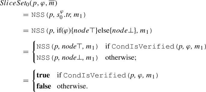
The truth values $\mathbf {true}$ and $\mathbf {false}$ are final once they are obtained, so this equation also holds for and leads to the following output:

figure al

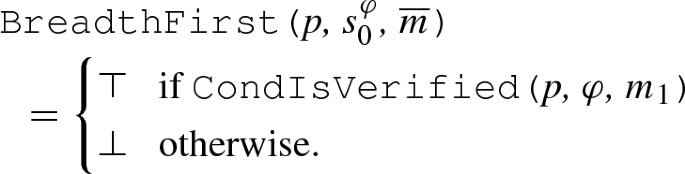
If $\varphi $ is an equality (resp. inequality), the condition evaluates to $p(x) = p(y)$ (resp. $p(x) \ne p(y)$), which is equal to $\varphi (p)$. Hence, the final output is equal to $[\overline{m} \models \varphi (p)] = [\overline{m} \models (p, \varphi )]$.

Induction step: For some integer $d \ge 0$, if Theorem 2 holds for any nonempty finite trace $\overline{m}$ and any well-formed couple $(p, \varphi )$ when $|\varphi | \le d$, then it also holds when $|\varphi | = d+1$.

Let $\overline{m} $ be some finite nonempty trace, and let $(p, \varphi )$ be a well-formed formula. Suppose $|\varphi | = d+1$. Since $d \ge 0$, $\varphi $ cannot be an equality nor an inequality; rather, it must take one of nine possible forms. If $\varphi $ is of the form $\exists _{\pi } x : \eta $, $\forall _{\pi } x : \eta $, $\mathbf{X\,}\, \eta $, $\mathbf{F\,}\, \eta $ or $\mathbf{G\,}\, \eta $, then the induction hypothesis covers $\eta $ because $|\eta | = d$. If $\varphi $ is of the form $\mu \vee \eta $, $\mu \wedge \eta $, $\mu \, \mathbf{\,U\,}\, \eta $ or $\mu \, \,\mathbf {R}\,\, \eta $, then it covers both $\mu $ and $\eta $ because $\max \{ |\mu |, |\eta | \} = d$.

For every form of $\varphi $, there exists an equation from Lemma 1 that, for all $0 \le i \le n$, links to SliceSets related to $\eta $ (and $\mu $). These equations, combined with the induction hypothesis, allow us to prove that returns $[\overline{m} \models (p, \varphi )]$. The details depend on $\varphi $, but it is always sufficient to show that returns $\top $ (resp. $\bot $) iff $[\overline{m} \models (p, \varphi )] = \top $ (resp. $\bot $) since these two equivalences imply that also returns $?$ iff $[\overline{m} \models (p, \varphi )] = \ ?$.

1.3.1 Case $\varphi = \mu \vee \eta $

Lemma 1 holds for any $1 \le i \le n$, so if $i = n$, we have

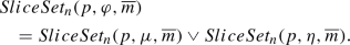
We previously observed that $|\mu | \le d$ and $|\eta | \le d$. Since $(p, \varphi )$ is well formed, $(p, \mu )$ and $(p, \eta )$ are also well formed and are covered by the induction hypothesis. It follows from this hypothesis, the equation above, and the Definition of LTL-FO$^+$ given in Definition 4, that

figure aq

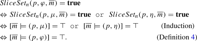
As a result, returns $\top $ iff $[\overline{m} \models (p, \varphi )] = \top $. A similar reasoning shows that returns $\bot $ iff $[\overline{m} \models (p, \varphi )] = \bot $. Thus, we can conclude that returns the correct value.

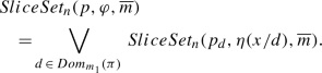
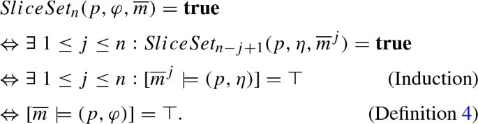
1.3.2 Case $\varphi = \exists _{\pi } x : \eta $

By Lemma 1, if $i = n$, then

We already established that $|\eta | \le d$ and that the couple $(p_{d}, \eta (x/d))$ is well formed. Therefore, the induction hypothesis covers $(p_{d}, \eta (x/d))$.

If $Dom_{m_1}(\pi )$ is empty, the disjunction in the equation above is conventionally set to $\mathbf {false}$, so . Otherwise, if $Dom_{m_1}(\pi )$ is not empty,

figure au

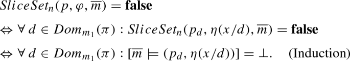
When we unify both scenarios, we get that iff 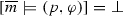(Definition 4). In other words, returns iff .

Similarly, iff there exists some $d \in Dom_{m_1}(\pi )$ for which (note that $Dom_{m_1}(\pi ) \ne \emptyset $ is implied). It follows from the induction hypothesis and Definition 4 that returns $\top $ iff $[\overline{m} \models (p, \varphi )] = \top $. Hence, returns the correct value.

1.3.3 Case $\varphi = \mathbf{X\,}\, \eta $

By Lemma 1, if $i = n$, then

If $n=1$, the last SliceSet computed by is $\{\{ (p, s_{\eta }^0) \}\}$. Since a verdict could not be assigned at that point, it evaluates to $?$, which is also the value of $[\overline{m} \models (p, \varphi )]$ (Definition 4). Otherwise, since $(p, \eta )$ is well formed and $|\eta | \le d$, we can use the induction hypothesis on . Doing so results in the desired equivalences:

(1)

(2)

Again, the output of is $[\overline{m} \models (p, \varphi )]$.

1.3.4 Case $\varphi = \mathbf{F\,}\, \eta $

By Lemma 1, if $i = n$, then

The SliceSet $\{\{ (p, s_0^{\varphi }) \}\}$ evaluates to $?$. As a result, the disjunction can never evaluate to $\mathbf {false}$,and will never return $\bot $. However, it returns $\top $ iff for some $1 \le j \le n$.

As with the previous case, the couple $(p, \eta )$ is well formed and $|\eta | \le d$. Also, for any $1 \le j \le n$, is the last term computed by . Therefore, we can use the induction hypothesis on this term and conclude that:

figure bc

In summary, never returns $\bot $ just like $[\overline{m} \models (p, \varphi )]$ is never equal to $\bot $, and it returns $\top $ iff $[\overline{m} \models (p, \varphi )] = \top $.

1.3.5 Case $\varphi = \mu \, \mathbf{\,U\,}\, \eta $

By Lemma 1, if $i = n$, then is equal to

figure be

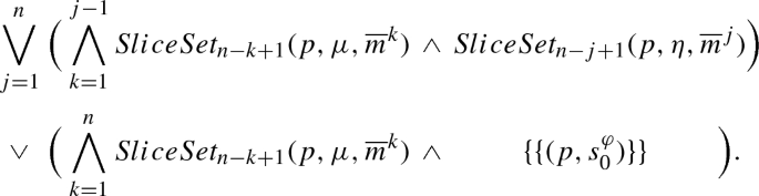
The couples $(p, \mu )$ and $(p, \eta )$, just like in the case $\varphi = \mu \vee \eta $, are well formed, and the size $|\cdot |$ of their formulae is less than or equal to d. Since the equation is a disjunction of conjunctions, is $\mathbf {true}$ iff one conjunction is $\mathbf {true}$. The SliceSet $\{\{ (p, s_0^{\varphi }) \}\}$ causes the last one to fail, so the results depend on the first n conjunctions:

figure bf

Thus, returns $\top $ iff $[\overline{m} \models (p, \varphi )] = \top $.

The following analogous reasoning can be used to show that returns $\bot $ iff $[\overline{m} \models (p, \varphi )] = \bot $. We omit it here out of space considerations:

A disjunction like is equal to $\mathbf {false}$ iff all its conjunctions are $\mathbf {false}$. In particular must admit a $\mathbf {false}$ term. Since $\{\{ (p, s_0^{\varphi }) \}\}$ evaluates to $?$, can only evaluate to $\mathbf {false}$ if fails for some $1 \le k \le n$. Let $k^*$ denote the smallest such value.

Let us now inspect every conjunction indexed by j where $j \le k^*$. Because $k \le j-1 < k^*$, any composing them is not $\mathbf {false}$ due to the minimality of $k^*$. However, the conjunctions themselves still fail, so must be $\mathbf {false}$ for all $j \le k^*$. In summary:

figure bi

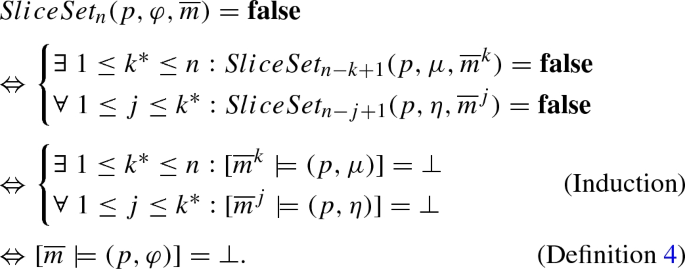
We showed that returns $\bot $ iff $[\overline{m} \models (p, \varphi )] = \bot $. Hence, returns the correct value.

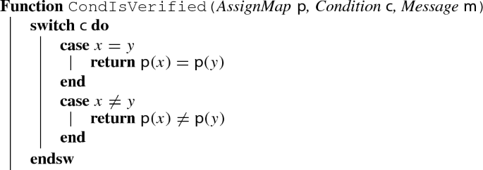
1.4 Function CondIsVerified

Function consults the valuation map and$\backslash $or the current message and determines whether a conditional expression holds. Boolean equality can easily be generalized to other connectives. Pelota currently supports equality and inequality between integers and strings as well as ‘<’ comparison between integers. We omitted the pseudocode of this function from the main paper out of space considerations, and due to its simplicity, but include it here for completeness.

figure bm

Automata-based monitoring for LTL-FO ^+$$ (original) (raw)

Appendix

1.1 Preliminaries

Definition 11

Theorem 2

1.2 Lemma on SliceSets

Definition 12

Lemma 1

1.3 Proof of correctness the main theorem

1.3.1 Case \(\varphi = \mu \vee \eta \)

1.3.2 Case \(\varphi = \exists _{\pi } x : \eta \)

1.3.3 Case \(\varphi = \mathbf{X\,}\, \eta \)

1.3.4 Case \(\varphi = \mathbf{F\,}\, \eta \)

1.3.5 Case \(\varphi = \mu \, \mathbf{\,U\,}\, \eta \)

1.4 Function CondIsVerified