Convergence Analysis in the Maximum Norm of the Numerical Gradient of the Shortley–Weller Method (original) (raw)
Abstract
The Shortley–Weller method is a standard central finite-difference-method for solving the Poisson equation in irregular domains with Dirichlet boundary conditions. It is well known that the Shortley–Weller method produces second-order accurate solutions and it has been numerically observed that the solution gradients are also second-order accurate; a property known as super-convergence. The super-convergence was proved in the \(L^{2}\) norm in Yoon and Min (J Sci Comput 67(2):602–617, 2016). In this article, we present a proof for the super-convergence in the \(L^{\infty }\) norm.
Access this article
Subscribe and save
- Starting from 10 chapters or articles per month
- Access and download chapters and articles from more than 300k books and 2,500 journals
- Cancel anytime View plans
Buy Now
Price excludes VAT (USA)
Tax calculation will be finalised during checkout.
Instant access to the full article PDF.
References
- Caffarelli, L.A., Gilardi, G.: Monotonicity of the free boundary in the two-dimensional dam problem. Annali della Scuola Normale Superiore di Pisa-Classe di Scienze 7(3), 523–537 (1980)
MathSciNet MATH Google Scholar - Chorin, A.J.: A numerical method for solving incompressible viscous flow problems. J. Comput. Phys. 135(2), 118–125 (1997)
Article MATH Google Scholar - Ciarlet, P.G., Miara, B., Thomas, J.M.: Introduction to Numerical Linear Algebra and Optimisation. Cambridge Texts in Applied Mathematics. Cambridge University Press, Cambridge (1989)
Google Scholar - Friedman, A.: Variational principles and free-boundary problems. Courier Corporation, North Chelmsford (2010)
Google Scholar - Gibou, F., Min, C.: Efficient symmetric positive definite second-order accurate monolithic solver for fluid/solid interactions. J. Comput. Phys. 231, 3245–3263 (2012)
MathSciNet MATH Google Scholar - Gustafsson, I.: A class of first order factorization methods. BIT 18, 142–156 (1978)
Article MathSciNet MATH Google Scholar - Harlow, F.H., Welch, J.E.: Numerical calculation of time-dependent viscous incompressible flow of fluid with a free surface. Phys. Fluids 8(3), 2182–2189 (1965)
Article MathSciNet MATH Google Scholar - Iserles, A.: A First Course in the Numerical Analysis of Differential Equations. Cambridge Texts in Applied Mathematics. Cambridge University Press, Cambridge (1996)
Google Scholar - Li, Z.-C., Hu, H.-Y., Wang, S., Fang, Q.: Superconvergence of solution derivatives of the shortley-weller difference approximation to poisson’s equation with singularities on polygonal domains. Appl. Numer. Math. 58(5), 689–704 (2008)
Article MathSciNet MATH Google Scholar - Ng, Y.T., Chen, H., Min, C., Gibou, F.: Guidelines for poisson solvers on irregular domains with dirichlet boundary conditions using the ghost fluid method. J. Sci. Comput. 41(2), 300–320 (2009)
Article MathSciNet MATH Google Scholar - Peskin, C.S.: Flow patterns around heart valves. In: Proceedings of the Third International Conference on Numerical Methods in Fluid Mechanics, pp. 214–221. Springer (1973)
- Shortley, G.H., Weller, R.: The numerical solution of Laplace’s equation. J. Appl. Phys. 9(5), 334–348 (1938)
Article MATH Google Scholar - Strikwerda, J.C.: Finite Difference Schemes and Partial Differential Equations. SIAM, New Delhi (2004)
Book MATH Google Scholar - Weynans, L.: A proof in the finite-difference spirit of the superconvergence of the gradient for the Shortley–Weller method. Ph.D. thesis, INRIA Bordeaux (2015)
- Xiu, D., Karniadakis, G.E.: A semi-Lagrangian high-order method for Navier–Stokes equations. J. Comput. Phys. 172(2), 658–684 (2001)
Article MathSciNet MATH Google Scholar - Yoon, G., Min, C.: Analyses on the finite difference method by Gibou, et al. for poisson equation. J. Comput. Phys. 280, 184–194 (2015)
Article MathSciNet MATH Google Scholar - Yoon, G., Min, C.: Convergence analysis of the standard central finite difference method for Poisson equation. J. Sci. Comput. 67(2), 602–617 (2016)
Article MathSciNet MATH Google Scholar - Yoon, G., Min, C., Kim, S.: A stable and convergent method for hodge decomposition of fluid-solid interaction. (2016). arXiv:1610.03195
Author information
Authors and Affiliations
- Ewha Womans University, Seoul, Republic of Korea
Jiwon Seo & Chohong Min - Seoul National University, Seoul, Republic of Korea
Seung-yeal Ha
Authors
- Jiwon Seo
- Seung-yeal Ha
- Chohong Min
Corresponding author
Correspondence toChohong Min.
Appendix: Detailed Calculations in Lemma 4.3
Appendix: Detailed Calculations in Lemma 4.3
In this section, we provide detailed calculations that lead to the estimate \(\left\| D_{x}^{h}c^{h}\right\| _{L^{\infty }\left( \tilde{\Omega _{o}^{h}}\right) }\le \frac{105}{4}\max _{\tilde{\Omega },\left| \alpha \le 5\right| }\left| \partial ^{\alpha }u\right| \cdot h^{2}\) in Lemma 4.3.
Using the Taylor series of \(u\left( x,y\right) \) at \(\left( x_{i+\frac{1}{2}},y_{j}\right) ,\) the terms that sum up \(D_{x}^{h}c^{h}\) in (4) are expanded. For notational conveniences, the local coordinates centered at \(\left( x_{i+\frac{1}{2}},y_{j}\right) \) are used in the calculations. For example, \(u_{i+1,j+1}\) is denoted by \(u\left( \frac{h}{2},h\right) \). The Taylor expansions are listed below with remainders.
\begin{aligned} \begin{array}{rrrrrrrrrrr} u\left( \pm \frac{3h}{2},0\right) =u &{} \pm &{} \frac{3h}{2}u_{x} &{} + &{} \frac{9h^{2}}{8}u_{xx} &{} \pm &{} \frac{9h^{3}}{16}u_{xxx} &{} + &{} \frac{27h^{4}}{128}u_{xxxx} &{} \pm &{} \frac{81h^{5}}{1280}u_{xxxxx}\left( \xi _{1}^{\pm },0\right) \\ u\left( \pm \frac{h}{2},0\right) =u &{} \pm &{} \frac{h}{2}u_{x} &{} + &{} \frac{h^{2}}{8}u_{xx} &{} \pm &{} \frac{h^{3}}{48}u_{xxx} &{} + &{} \frac{h^{4}}{384}u_{xxxx} &{} \pm &{} \frac{h^{5}}{3840}u_{xxxxx}\left( \xi _{2}^{\pm },0\right) \end{array}\\ \begin{array}{rrrrrcc} \Delta u\left( \pm \frac{h}{2},0\right) =\Delta u&\pm&\frac{h}{2}\left( u_{xxx}+u_{xyy}\right)+ & {} \frac{h^{2}}{8}\left( u_{xxxx}+u_{xxyy}\right)&\pm&\frac{h^{3}}{48}\left( u_{xxxxx}+u_{xxxyy}\right) \left( \xi _{4}^{\pm },0\right) \end{array} \end{aligned},canceledoutallthetermsbuttheremainders.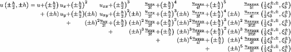
When the above expansions are inserted into the summation of \(D_{x}^{h}c^{h}\), canceled out all the terms but the remainders.,canceledoutallthetermsbuttheremainders.\begin{aligned} D_{x}^{h}c_{i+\frac{1}{2},j}^{h}{=}\frac{h^{2}}{120}\left( \begin{array}{l} {-}\left( \frac{3}{2}\right) ^{5}\left( u_{xxxxx}\left( \xi _{1}^{+},0\right) {+}u_{xxxxx}\left( \xi _{1}^{-},0\right) \right) {+}\frac{5}{2^{5}}\left( u_{xxxxx}\left( \xi _{2}^{+},0\right) {+}u_{xxxxx}\left( \xi _{2}^{-},0\right) \right) \\ -\left( \frac{1}{2}\right) ^{5}\left( \begin{array}{r} \left( u_{xxxxx}{+}u_{xxxxy}{+}u_{xxxyy}{+}u_{xxyyy}{+}u_{xyyyy}{+}u_{yyyyy}\right) \left( \frac{1}{2}\xi _{3}^{+,+},\xi _{3}^{+}\right) \\ {+}\left( u_{xxxxx}{-}u_{xxxxy}{+}u_{xxxyy}{-}u_{xxyyy}{+}u_{xyyyy}{-}u_{yyyyy}\right) \left( \frac{1}{2}\xi _{3}^{+,-},\xi _{3}^{-}\right) \\ {+}\left( u_{xxxxx}{-}u_{xxxxy}{+}u_{xxxyy}{-}u_{xxyyy}{+}u_{xyyyy}{-}u_{yyyyy}\right) \left( \frac{1}{2}\xi _{3}^{-,+},\xi _{3}^{+}\right) \\ {+}\left( u_{xxxxx}{+}u_{xxxxy}{+}u_{xxxyy}{+}u_{xxyyy}{+}u_{xyyyy}{+}u_{yyyyy}\right) \left( \frac{1}{2}\xi _{3}^{-,-},\xi _{3}^{-}\right) \end{array}\right) \\ +\frac{5}{2}\left( \left( u_{xxxxx}+u_{xxxyy}\right) \left( \xi _{4}^{+},0\right) +\left( u_{xxxxx}+u_{xxxyy}\right) \left( \xi _{4}^{-},0\right) \right) \end{array}\right) \end{aligned}Now,weprovethelemma.Now, we prove the lemma.Now,weprovethelemma.\begin{aligned} \begin{array}{rcl} \left| D_{x}^{h}c_{i+\frac{1}{2},j}^{h}\right| &{} \le &{} \max _{\tilde{\Omega },\left| \alpha \right| \le 5}\left| \partial ^{\alpha }u\right| \cdot \frac{h^{2}}{120}\left( 2\cdot \left( \frac{3}{2}\right) ^{5}+2\cdot \frac{5}{2^{5}}+4\cdot 6\cdot \left( \frac{1}{2}\right) ^{5}+2\cdot 2\cdot \frac{5}{2}\right) \\ &{} = &{} \frac{105}{4}\max _{\tilde{\Omega },\left| \alpha \le 5\right| }\left| \partial ^{\alpha }u\right| \cdot h^{2}. \end{array} \end{aligned}$$
Rights and permissions
About this article
Cite this article
Seo, J., Ha, Sy. & Min, C. Convergence Analysis in the Maximum Norm of the Numerical Gradient of the Shortley–Weller Method.J Sci Comput 74, 631–639 (2018). https://doi.org/10.1007/s10915-017-0458-z
- Received: 10 April 2017
- Revised: 05 May 2017
- Accepted: 15 May 2017
- Published: 27 May 2017
- Issue date: February 2018
- DOI: https://doi.org/10.1007/s10915-017-0458-z