Transmission intensity and impact of control policies on the foot and mouth epidemic in Great Britain (original) (raw)
Data Sources and Links
DCS Database
Data were downloaded from the Disease Control System (DCS) database created and maintained by DEFRA (formerly MAFF). This database included both epidemiological and management data on every farm identified as being affected by FMD (IPs) as well as farms culled in the control of the FMD epidemic. For each IP, we extracted data on the dates of disease report, confirmation and cull, the number of cattle, pigs and sheep, and the point location of the farm. For each farm culled for disease control, we extracted data on the date that culling was completed, the numbers of cattle, pigs and sheep culled, the scheme under which the farm was culled and the point location of the farm. Where multiple entries for the same farm appeared in the database, identical duplicate records were first eliminated, and from the remainder numbers of animals were taken to be the maximum number recorded as "slaughtered" or "on farm". Where multiple slaughter dates appear, the analysis uses the date on which the largest number of animals is recorded to have been slaughtered (except for IPs where the last slaughter date is used). The 1849 FMD case confirmed up to July 16th 2001 were used in this analysis. A total of approximately 5600 unique CPH numbers were listed in the DCS database for farms culled under the various non-IP culling programmes up to that time (excluding records where no cull date was present), and an additional 240 farms were listed as having been slaughtered on suspicion of FMD infection but where later infection was not confirmed.
VLA FMD Case Database
Data on the farms affected by FMD (IPs) were provided by the Veterinary Laboratory Agency (VLA) epidemiology group. Since many variables also appeared in the DCS database, this database was only used for the estimated date of infection for each IP. Our earlier work1, including the estimated spatial kernel plotted in Fig. 2a was based DEFRA-identified infectious contacts, utilized this database for all FMD-related information about IPs.
Census Database
Data from June 2000 Agricultural and Horticultural Census11 were provided by Ministry of Agriculture, Fisheries and Food, the National Assembly for Wales Agriculture Department and the Scottish Executive Rural Affairs Department (Crown copyright 2001). We utilized farm-specific data on point location, farm land area and the numbers of cattle, pigs and sheep. Approximately 131,000 livestock farms with cattle, sheep and/or pigs were included in this dataset. It should be noted that sampling was introduced from 1995 for over 35,000 smaller holdings (many without livestock), and these then only received a census form once every three years. Thus while the datasets provided by DEFRA and the Scottish Executive provided comprehensive coverage of all livestock farms in GB, data on livestock numbers will have been based on earlier census years for farms without a June 2000 return (either due to sampling or other non-receipt of a completed form).
It should also be noted that since completion of the analyses in this paper, data from the Cattle Tracing System (originally launched in 1998, with all cattle in Great Britain registered by the end of 2000) has been received, giving details of the number of cattle at each holding in GB as at 28 February 2001. These data (unfortunately unavailable for other species) give the most accurate and timely picture of the national cattle herd available. Cross-linking with the census database revealed that the June census reports of cattle numbers were highly predictive of the number on farm in February 2001, thus providing validation (for cattle at least) of the use of census data in estimating farm stock levels within the analyses in this paper.
LW(D)S Database
The Livestock Welfare (Disposal) Scheme (LW(D)S) was designed to relieve the animal welfare problems resulting from FMD-related restrictions on animal movements. The Intervention Board provided data on date of cull, the species and number of animals culled for each farm on which animals were culled under the LW(D)S.
Farm Fragmentation Database
Integrated Administration and Control System (IACS) data on land parcels associated with each farm in Great Britain were analysed by the Farming and Rural Conservation Agency. They created a database of disconnected land parcels (each could consist of multiple fields, for example) by estimating contiguity using a Voronoi tessellation based on parcel centroids. In the analyses presented here, we used the estimated number of disconnected land parcels associated with each farm. However, due to inconsistencies in how land parcels are recorded in the database systems in Scotland and the rest of Great Britain, estimates of average numbers of disconnected land parcel drop sharply at the English/Scottish border. For that reason the risk estimates for Scotland are not directly comparable to those for England and Wales, and are not therefore plotted in the risk maps. Scottish data was however used in estimating the risk coefficient associated with fragmentation in the spatial hazard model: excluding this data from the analysis gave substantially greater estimates of the impact of fragmentation to farm susceptibility.
Integrated Database
The data from the first four sources were linked together using the county-parish-holding (CPH) unique farm identifier to form an integrated database of farms with cattle, sheep and/or pigs. In general, approximately 75% of farms listed in the DCS database could be matched to census farms, due to inconsistencies in recorded CPH number between the different sources. The proportion of matches was even lower for the LW(D)S database, where many more temporary holding numbers were used. However, even when farms could not be linked to census data, they were still included in the integrated database. The farm fragmentation dataset was used to obtain the number of disconnected land parcels for farms in this integrated database, though again this could only be achieved for approximately 75% of farms due to mismatches in CPH codes between IACS and census data. The number of land parcels for farms with missing farm fragmentation data was estimated using the farm-type- and county-specific averages.
Data on point location and numbers of animals by species appeared in more than one database. The location data in the DCS database was regarded as the most reliable, with locations from the census database used in all other cases. Farms without point location data could not be included in the neighbourhood calculations. The numbers of animals by species were estimated from the maximum recorded for each farm on the DCS, census and LW(D)S databases.
The contiguous premises (CPs) of each IP were identified using approximated farm boundaries obtained using the Quickhull algorithm15 for constructing Voronoi diagrams from the point locations of farms reported in the June 2000 agricultural census11. This approach is clearly less optimal than precise identification of farm neighbours, but unfortunately no integrated database of farm boundaries exists of sufficient detail to allow such an approach to be used. Indeed, in implementing the CP culling programme, DEFRA have made judgements of contiguity on the ground on a case by case basis. In performing our approximate analysis, we used freely available Qhull 3.0 software at http://www.geom.umn.edu/locate/qhull. We chose not to use the fragmentation data to identify CPs (e.g. on the basis of any parcel contiguous to any IP parcel) because only farms contiguous with the parcels containing infected animals are typically designated as CPs for culling purposes, meaning a single farm basis is the best analytical approximation possible for judging contiguity in the context of CP culling.
Parameter Estimation
Symbol definitions
a_k_:
relative infectiousness of farms in class k;
t_l_:
relative susceptibility of farms in class l;
θ:
linear effect of farm fragmentation on susceptibility;
l:
susceptibility scaling factor;
nIP:
total number of IPs;
d kli:
day on which farm {k l i} was infected;
η kli (d):
relative infectiousness of a farm {k l i} d days after infection;
f {kli}{k'l'j}:
probability that infected farm {k l i} was infected by farm {k' l' j};
d {kli}{k'l'j}:
distance between farms {k l i} and {k' l' j};
r(d):
relative infectiousness of an infected farm to a susceptible farm distance away;
b D:
transmission coefficient on day D;
w{k' l' j}{kl}(D):
susceptibility-weighted neighbourhood of farm {k' l' j} consisting of farms in infectiousness class k and susceptibility class l that remains on day D;
X̅ IP:
mean number of disconnected land parcels associated with IPs;
Ψ {kli}{k'l'j} (D):
probability that farm {k' l' j}infected farm {k l i} on day D;
N(D):
total number of infections that occurred on day D;
r k’ l' j:
relative transmission risk of farm {k' l' j} to surrounding farms.
Indicator variables
K kli (D):
1 if farm {k l i} remains susceptible (not culled or infected with FMD) on day D and 0 otherwise;
 :
:
1 if farm {k l i} is in 5km square q and 0 otherwise;
Estimation of transmission and susceptibility parameters
Farms are indexed by the triple {k l i} with k and l respectively denoting farm-type-dependent infectiousness and susceptibility classes, and i indexing farms within the {k l} class. The relative infectiousness of farms in infectiousness class k is denoted a k. Similarly, the relative susceptibility of farms in infectiousness class l is denoted t l. Furthermore, we assume that relative susceptibility is linearly related to the number of land parcels (x kli for farm {k l i}) such that the relative susceptibility of farm i is proportional to: (1+θx kli). The relative susceptibility of farm i in infectiousness class k and susceptibility class l is thus given by:

where l is the scaling factor required to have the sum of infections weighted by the inverse of susceptibility equal the observed number of infections (i.e. the number of IPs, denoted n IP), such that

where k, l and i are summed over all IPs.
We have constructed the model in a general form allowing for variable infectiousness, η kli(d), as a function of days, d, since infection on farm{k l i}. However, for simplicity, in the results presented we assumed that infectiousness does not vary from the day after infection until the date on which the farm was culled. Thus, for farm {k l i} infected on day d kli, η kli(D-d kli)=1 for D>d kli and D less than the cull date of that farm, and 0.
Due to the lack of certainty in the source of most farms’ infections, source farms are attributed probabilistically based on their relative infectiousness to the reference farm on the day it was recorded as having been infected. Thus, the probability that infected farm {k l i} was infected by farm {k' l' j}, denoted f {kli}{k'l'j} and alternatively viewed as the proportion of the infection of farm {k l i} attributed to farm {k' l' j}, is estimated as:
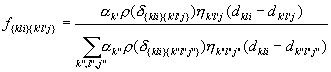
where {k'' l'' j''} labels all of the farms that could have infected farm {k l i}and r(d {kli}{k'l'j}) is the relative infectiousness of an infected farm to a susceptible farm distance d {kli}{k'l'j} away (normalised such that its sum over all distance categories is 1). The farm-specific estimate of the effective reproduction number (R k'l'j) is then obtained by summing the proportions of infections attributed to each farm weighted according to their susceptibility, such that

where {k l i} indexes IPs potentially infected by farm {k' l' j}.
The farm-specific  value requires a correction for neighbourhood depletion such that

where {k l i} indexes IPs potentially infected by farm {k' l' j}. w{k' l' j}{kl}(D) is the susceptibility-weighted neighbourhood of farm {k' l' j} consisting of farms in infectiousness class k and susceptibility class l that remains on day D and is given by:

where {k l i} indexes all other farms, and K kli (D) =1 if farm {k,l,i} remains susceptible (not culled or infected with FMD) on day D and 0 otherwise.
Initially it is assumed that all categories of farm are equally infectious and susceptible (i.e. a_k_=t_l_=1 for all k and l and θ=0) and starting values are chosen for  . These parameters are estimated iteratively until convergence of all infectiousness, susceptibility and spatial kernel parameters.
The transmission coefficient for day D, b D, is estimated to be the average day-specific contribution to  , the average of the IP-specific
  values, such that:

The farm-type-dependent infectiousness and susceptibility parameters (a k and t l) are estimated by solving the equations obtained by equating the observed and predicted number of infections in each (infectiousness or susceptibility) class:

for each k' and

for each l. Here c a and c t are normalisation constants such that the infectiousness and inverse susceptibility averaged across all IPs are 1. In each case, both {k l i} and {k' l' j} index all IPs.
The spatial kernel was similarly estimated by discretising the distances between farms such that the relative infectiousness of an infected farm to a susceptible farm distance d away, r(d) is estimated from the equations of the following form:

where d m is the _m_th category of distance determining the estimated relative infectiousness between infectious and susceptible farms, c a is a normalisation constant such that r(_d_0)=1, and both {k l i} and {k' l' j} index all IPs.
The effect of farm fragmentation, θ, is estimated by solving the equation derived by equating the expected number of fragments in the farms infected by IPs over the course of the epidemic with the observed average number of fragments among IPs:

where {k' l' j} indexes IPs, {k l i} indexes all susceptible farms and X̅ _IP_is the mean number of disconnected land parcels associated with IPs.
The infectiousness, susceptibility and spatial kernel parameters are re-estimated iteratively until convergence.
The likelihood of the observed epidemic can be calculated based on the farm-type, fragmentation and locations of each farm in the country. For each day, the infection probabilities are obtained from the estimated hazards scaled to sum to the observed number of infections. Thus, the infection hazard from farm {k' l' j} to farm {k l i} on day D is given by

where N(D) is the total number of infections that occurred on day D, {k l i} indexes all farms and {k' l' j} indexes all infectious farms. Hence, the log likelihood of farm {k l i} not being infected by day D 0 is approximated by:

and the log likelihood for farm {k l i} being infected on day D 1 is given by:

Likelihood-based hypothesis tests and confidence intervals are then obtained using the result that twice the difference in the full log likelihood will be chi-squared distributed with degrees of freedom equal to the number of constrained parameters.
A full likelihood-based estimation procedure was not pursued due to the prohibitive computational burden that would have been involved in simultaneously estimating the parameters relating to time-varying infection risk, variable infectiousness and susceptibility of farms and the spatial kernel. However, the estimates obtained, using the equations given above, were very close to the maximum likelihood estimates and always lay within parameter confidence bounds calculated with respect to maximum likelihood point of univariate profile likelihoods.
Risk Maps
The risk maps are constructed by estimating a measure of relative transmission risk from each farm {k' l' j} to surrounding farms, r k' l' j, such that:

where {k l i} indexes all farms in Great Britain. To obtain the average transmission risk in each 5km square in the country, the r k' l' j values are averaged weighting by the susceptibility of farm {k' l' j}, since a more susceptible farm is more likely to become infected and thus transmit infection. Hence, the mean transmission potential for a 5km square in the country is estimated by:
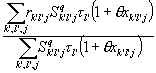
where {k' l' j} indexes all farms in Great Britain and  equals 1 if farm {k' l' j} is in 5km square q and 0 otherwise.
Similarly, farm density and fragmentation level averages were smoothed using the spatial kernel, such that the mean number of farms in a 5km square was calculated as
and the average fragmentation of farms in a 5km square as

Enlarged copy of Figure 2C
Given the importance of the results shown in fig 2C to later analyses and the limited space available in the main text, we reproduce this figure here at a larger scale.
